Getting information from your graph
It is often useful to either identify a particular data point on a graph (because we might be interested in other variables attached to this record or find outliers for example) or to simply locate a particular point by getting its coordinates. R offers the possibility to do that by conveniently using your mouse.
The function “identify()” will allow you to determine which record correspond to a particular data point on the graph, simply by clicking on it. In order to do that, we first need to call the graph (with the plot function for example), and then call the “identify()” function. We have to let the function know the data we are working with (i.e. the coordinates we are using). This can be done using the same formulation as with the “plot()” function. Finally, we can either decide to let the function know that we want to identify a certain number of points by setting the argument “n” to the said number of points we want to identify; or we can not specify anything and simply use the right-click when we’re done.
plot(student~mother,data=size)
identify(size $student~ size $mother)   # Right-click method
[1]  21  67 113
identify(size $student~ size$mother,n=2)   # We only need to identify two data points
[1]  21  67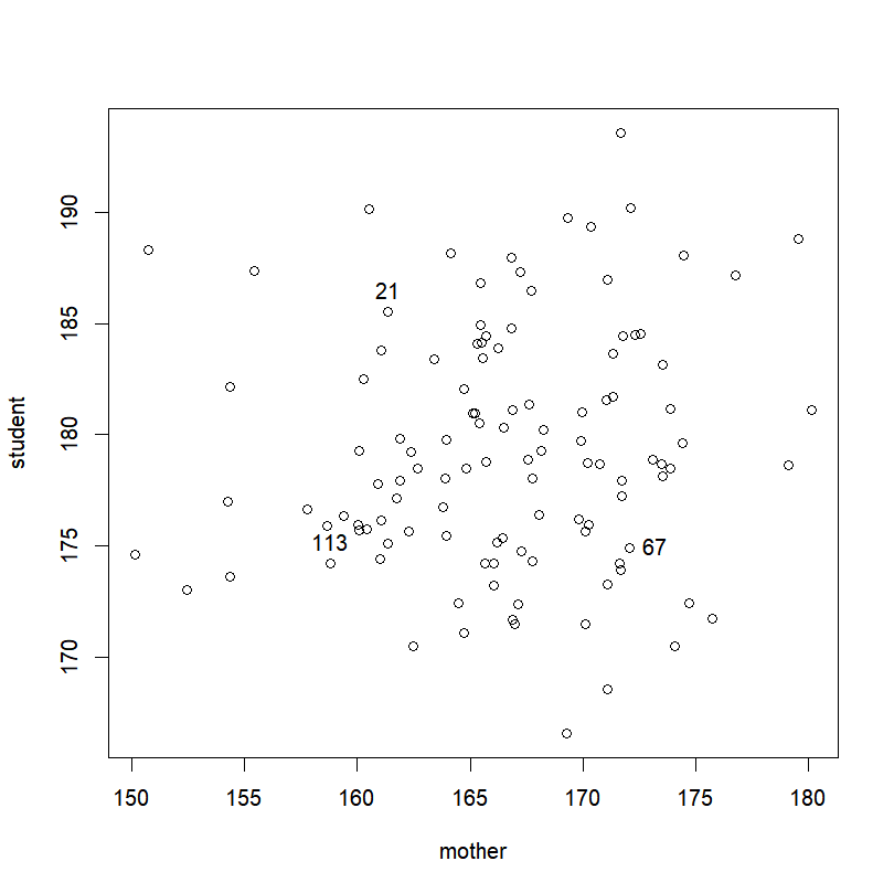
The function returns a vector of the IDs of the points identified, as well as labels them on the plot (this last option can be removed). This can be stored and used to access the corresponding raw data. E.g.:
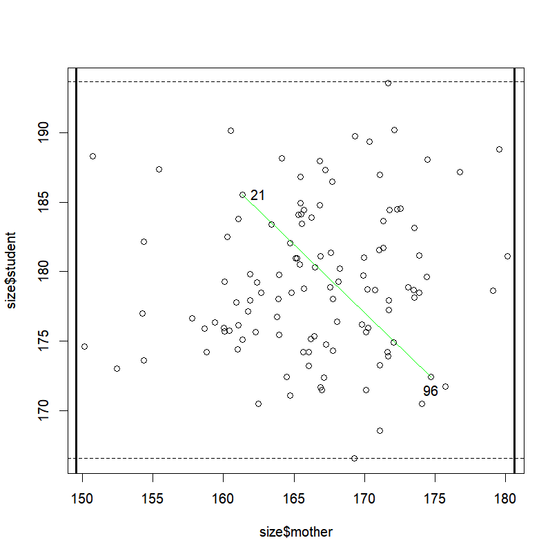
plot(size$mother,size$student)
whoisthat=identify(size$mother,size$student,n=2)   # We only need to identify two data points
We can now use this to extract information about those students:
size[whoisthat,]
     father  student   mother
47 179.8075 176.2877 154.8316
88 171.5993 183.6219 179.1695
If you are only interested in finding the coordinate of a particular area/point in the window, the function “locator()” will help you. While “identify()” can only find points that are in your input dataset, “locator()” will find coordinates for any point clicked on the active graph. In this case, you can simply call the function. No need to feed it with our data. As we “identify()”, we can let the function know that want to record a particular number of points (by setting the argument “n” to the said number of points); or we can not say anything and simply use the right-click when we’re done.
locator() # Right-click method
$x
[1] 154.0573 167.2716 174.2901 155.3184
$y
[1] 183.9697 190.6053 167.4069 166.6754
locator(n=2)  # We just want to get 2 points (output not shown)
locator(2)  # Alternative formulation  (output not shown)
As you can see, the function returns a list with 2 components. They are named “x” and “y”, and correspond to the x-coordinate, and the y-coordinate respectively.
Exercise 4.1> – plot the size of students against the size of their mother
|
MORE GRAPHICAL FUNCTIONS
Want a histogram? A boxplot? A barplot? You came to the right place!
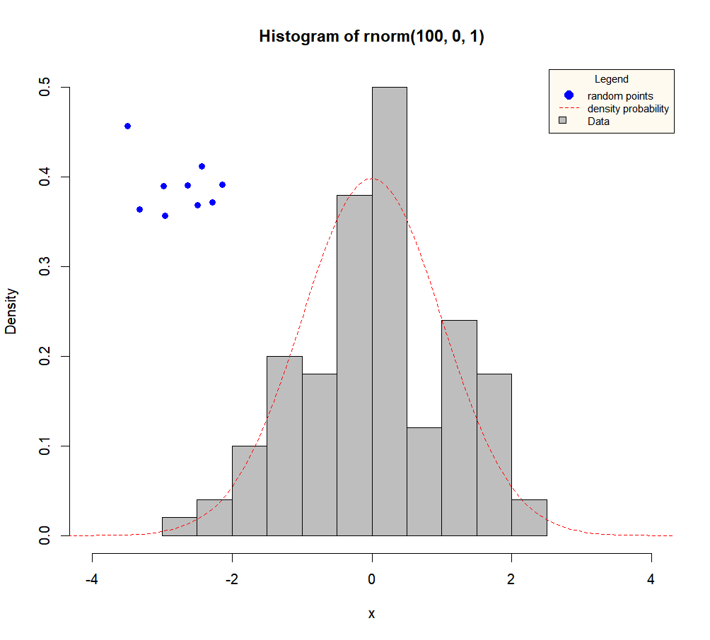
THE “PLOT()” FUNCTION
A picture is worth a thousand words. Here is how to make a graph worth twice that.
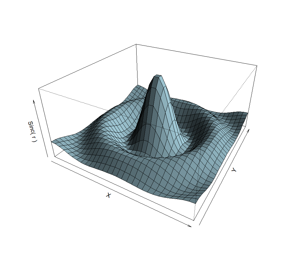
A LITTLE BIT OF 3D?
2D is so 1990. 3D is the future.
ADDING ELEMENTS
A look at putting finishing touches to your masterpiece.