Basic statistics
Let’s assume for a minute that you would like to study the average size of students, based on their sex and a random sample of 10 men and 8 women. Here are our data: (in the metric system, because the imperial system sucks)
men = c(172.5, 175, 176, 177, 177, 178.5, 179, 179, 179.5, 180)
women = c(167, 168, 168.5, 170, 171, 175, 175, 176)
In order to know the mean, the variance, the standard deviation or simply check the size of our sample, we can respectively use the functions:
mean(men)
[1] 177.35
var(men)
[1] 5.502778
sd(men)
[1] 2.3458
length(men)
[1] 10
If your dataset contains NAs (i.e. missing values), you can let R know to remove them by setting the argument “na.rm” to True in any of those functions (except “length()”).
tmpNA=c(2,1,3,4,1,2,3,NA)
mean(tmpNA)
[1] NA
mean(tmpNA,na.rm=T)
[1] 2.285714
When dealing with matrices or arrays, “mean()” and “sum()” will give the mean/sum for the whole dataset. If you are interested in the mean and sum of each row, or each column, you can use the functions “rowMeans()”, “colMeans()”, “rowSums()” or “colSums()” instead. Side note, R doesn’t readily include a function to give the standard error (that I know of at least). You can simply apply the formula for the standard error to calculate it yourself:
sqrt(var(men)/length(men))
[1] 0.7418071
We’ll see in a later chapter how to create our own function to realize this task. Equally, if we would like to get the median, the maximum or minimum values, or even the range, we simply need to use the functions:
median(women)
[1] 170.5
max(women)
[1] 176
min(women)
[1] 167
range(women)
[1] 167 176
It is interesting to note that R doesn’t readily come with a function to estimate the mode of a dataset. Well, some people thought it could be interesting, so they developed a function for that. Remember how I told you that “if you can think of it, you can create (or find) a function that will do it!”? No? Well, you should! So, somebody decided to create this function in R. And not only did they create it, but they also made it available to other R users. In order to do that, they “packaged” several functions together, and made it available on CRAN’s website. We’ll see how we can use that to make our life easier.
First, click on “Packages” at the top of your screen, then go to “Install package(s)…” and select the CRAN mirror the closest to your location in the window that will appear. After clicking on “OK”, you can highlight the package(s) you want to install. For now, let’s only take care of a package called “modeest“. Scroll down, select it, and click OK. R will download the corresponding file, and save it in its library (a folder with all the packages you have ever installed). Now that it is downloaded, we still need to load it in our R session. To do so, we can simply call it with the functions “library()” or “require()”.
library(modeest)
This is package 'modeest' written by P. PONCET.
For a complete list of functions, use 'library(help = "modeest")' or 'help.start()'.
Warning message:
package ‘modeest’ was built under R version 3.0.2
Done? You should now have access to the function “mlv()” that will allow you to compute the mode of your dataset:
mlv(men, method = "mfv")
Mode (most likely value): 178
Bickel's modal skewness: 0
Call: mlv.default(x = men, method = "mfv")
The argument here is only to specify the way we want to estimate the mode. To have an overlook of the other methods available, simply look at the help file for this function. Remember how? As you can see by calling the data “women”, R keeps the values in the object in the same order they were entered. Now, if that doesn’t suit you, you can reorder your vector in an ascending or descending order:
sort(women)
[1] 167.0 168.0 168.5 170.0 171.0 175.0 175.0 176.0
sort(women, decreasing = T)
[1] 176.0 175.0 175.0 171.0 170.0 168.5 168.0 167.0
(For data frames, use the function “order()“) And if for whatever reason, you are curious how high your sample would go if they were circus performers and standing on each other’s head, you can sum the elements of a vector:
sum(men)
[1] 1773.5
sum(women,men)
[1] 3144
When dealing with data frames, some other information might be relevant. Similar to the “length()” function, we can get the dimension of a data frame or matrix:
dim(shirts)
[1] 6 2
dim(bear)
[1] 3 4
Or if you are simply interested in the number of rows, or columns:
nrow(bear)
[1] 3
ncol(bear)
[1] 4
It is also possible to get or set the headers for the rows and columns of a matrix-like object:
colnames(shirts)
[1] "color"       "awesomeness"
colnames(shirts)<-c("hue","perfectness")
colnames(shirts)
[1] "hue"         "perfectness"
Or to get or set the names of the elements composing a list or vector (it can also be used for matrices):
names(data)
[1] "shirts"      "students"    "somerawdata"
To get an idea of how our data are internally structured, we can easily look at a contingency table of the counts at each combination of factor levels. This works well for vectors too.
table(shirts)
            perfectness
  hue        3 4 6 7 9
  orange     0 0 0 1 0
  peach puff 0 0 1 0 0
  pink       0 1 0 0 0
  powderblue 1 0 0 0 0
  salmon     0 0 0 0 1
  salmon2    0 0 0 0 0
And finally, talking about structure, the first step to take (and therefore presented last here) when trying to get information about what is in an object: the function “str()” will allow you to conveniently display the internal structure of an R object. It offers a nice alternative to summary while giving a little bit more information. As with “summary()“, the type of information that will be displayed depends on the type of object studied.
str(shirts)
'data.frame':   6 obs. of  2 variables:
 $ hue        : Factor w/ 6 levels "orange","peach puff",..: 5 1 3 4 6 2
 $ perfectness: num  9 7 4 3 NA 6
str(vec)
num [1:5] 2 3 10 -5 -0.33
str(women)
num [1:8] 167 168 168 170 171 ...
Exercise 2.1 – If not already done during chapter 1, create 2 vectors named ‘vecA’ and ‘vecB’ of any 10 positive numbers.
Answer 2.1
[collapse]
|
INTRODUCTION
The core of what we're doing is R is dealing with data. Let's see how to play with it for a bit.
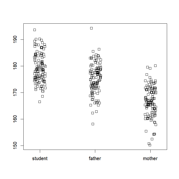
A QUICK LOOK AT OUR DATA
Basic plots for data exploration.
ACCESS, EXTRACT AND MERGE DATA?
a.k.a. Data management 101
CONCLUSION
The return of the sequel…