Correlation

Correlation

 

Computing the strength of the relationship between two quantitative variables normally distributed in regard to each other: Pearson’s R

If the two variables are bivariately normally distributed, it is possible to use Pearson’s product-moment correlation, also called Pearson’s R. What it means is that if one variable is fixed, the other one should be normally distributed. Practically, this assumption is met most of the time when dealing with a lot of data (as usual).

The correlation coefficient will vary between 1 (perfect positive correlation) and -1 (perfect negative correlation). A coefficient of 0 indicates that there is no correlation.

Let’s take an example. I like examples, they examplify things well.

So, a cook named James does his best to win a Chili cook-off. We have recorded his rank in regard to the amount of spices he put in his chili. Should we look at the correlation between those two variables?

rank=c(1,5,10,15,20)
spice=c(50,20,25,7,3)
plot(spice,rank)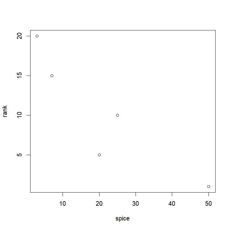

It is easy to obtain the correlation coefficient:

cor(spice,rank)
[1] -0.8972387

Wow, that’s pretty good isn’t it? A correlation of -0.897! It must definitely mean that the more spice James puts in his chili, the better it is!

But, wait a minute platypus! Is it really significantly different from 0? It might sound like a stupid question, but we are dealing with little data here. Let’s test this:

cor.test(spice,rank)
       Pearson's product-moment correlation
data:  spice and rank
t = -3.5196, df = 3, p-value = 0.03893
alternative hypothesis: true correlation is not equal to 0
95 percent confidence interval:
 -0.99324714 -0.07184525
sample estimates:
       cor 
-0.8972387 

Haha. Well, yes, this test is statistically significant with a p-value of 0.03893. But look at the 95 percent confidence interval. Our “true” correlation coefficient is almost certainly between -0.993 and -0.072… It could be as “low” (i.e. as close to zero) as -0.072. In turn, to see the strength of the relationship (a.k.a. coefficient of determination or R-squared), we need to square this value. The coefficient of determination gives you the fraction of variance explained by the model.

-0.072^2
[1] 0.005184

0.005184…. 0.5%… In this case, if we fix one parameter (amount of spice), we’ll be able to reduce the variability of the other (what rank James is likely to obtain) by a whopping 0.5%…

---

Computing the strength of the relationship between two quantitative variables non normally distributed in regard to each other: Spearman’s R

In the case you’re dealing with data that are not bivariately normally distributed, you need to use Spearman’s rank correlation (aka Spearman’s R), especially if dealing with little data. To do so, you simply need to specify to the function cor.test that you want to use Spearman’s method in the function’s arguments:

cor.test(spice,rank,method="spearman")
        Spearman's rank correlation rho
data:  spice and rank
S = 38, p-value = 0.08333
alternative hypothesis: true rho is not equal to 0
sample estimates:
 rho 
-0.9 

As you can see here, by removing one constraint, we are losing power in our test and are not detecting a statistically significant correlation coefficient.