The “plot()” function
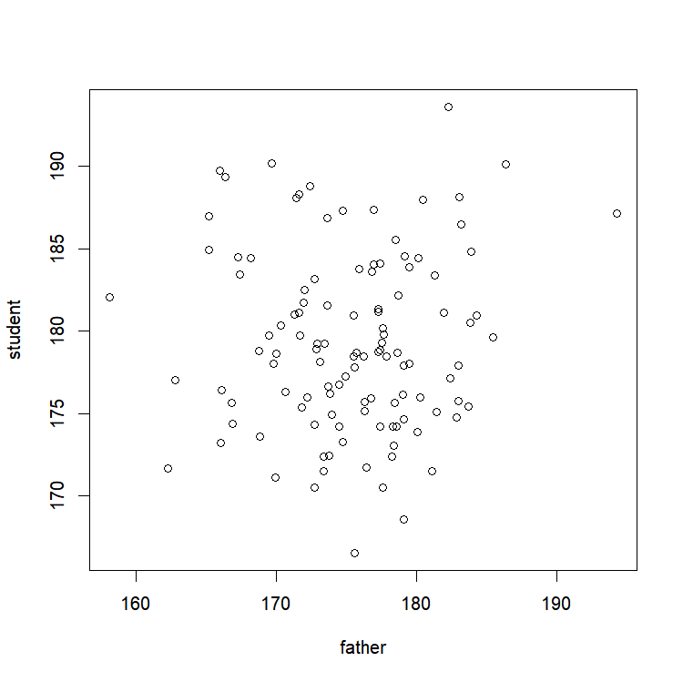
Remember the most basic instruction for plotting data? An easy way to represent a quantitative variable Y in function of another variable X? Let’s look at our students and parents’ size.
To use the “plot()” function, we can give it the coordinates for the different points to display in several ways:
1/ By giving the coordinates in 2 separate vectors:
plot(x=father,y=student)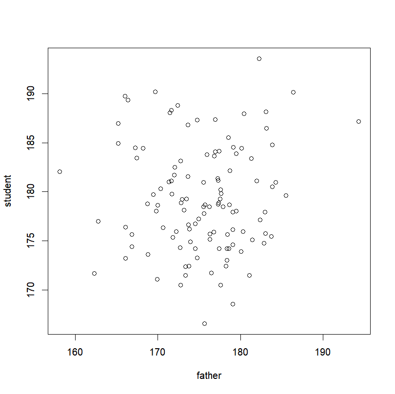
equivalent to
plot(father,student)[same graph as above!]
2/ By using a data frame:
If the data frame contains only 2 columns, by default, R will take the first one as the X-coordinates, and the second one as the Y-coordinates.
size=data.frame(father,student)
plot(size)
[bis repetita, same graph as above!]
If the data frame contains more than 2 columns, you will have to either specify which columns should be used,
size=data.frame(father,student,mother)
plot(size[,c(1,2)])
[again, same graph as above!]
or R will plot the plots for all the possible combinations of columns,
plot(size)
3/ You can also use the formula formulation:
With vectors:
plot(student~father)[seriously, you’re not getting tired? same graph as the one seen just a second ago!]
Or with a dataframe (in this case don’t forget to let R know where he should take the data from):
plot(student~father,data=size)[arghhh!!! Again…]
4/ Or finally, in some cases, the results from a function:
plot(lm(student~father))
At this point in space and time, you should be in awe at how easy it is, and at how nice the default features are. You should also have noticed that the axes are already labelled, but that our graph is missing a title, and that it’s a little dark, and also possibly you don’t like the circles for your points, and other stuff. Ok, no problem, we can modify that by feeding arguments in the plotting function. There are literally dozens and dozens of possible of arguments that can be used. I’ll present a few below, but if you’re curious you can look at the help of the “plot()” function, and also at the parameters presented in the “par()” function’s help.
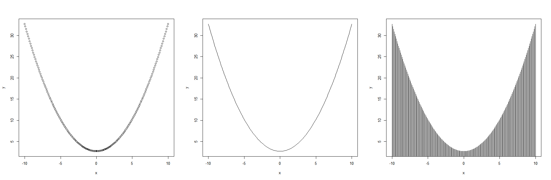
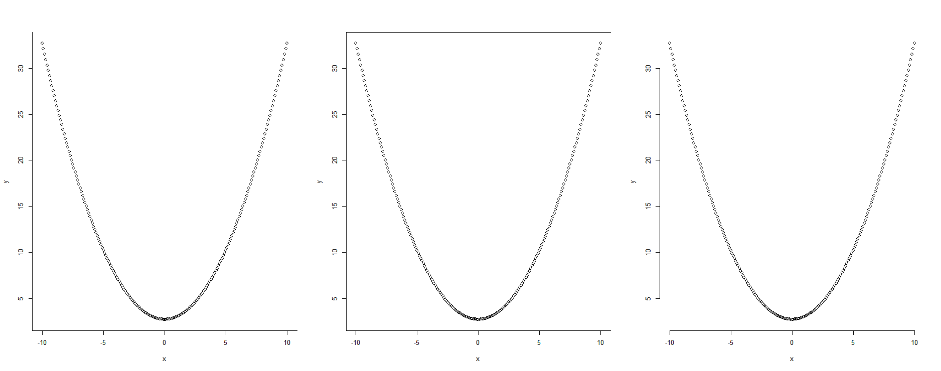
Don’t like the style of the points? You can change them by setting the argument “type” to points (“p”), lines (“l”) or to histogram-like vertical lines (“h”). (As previously said, other options are available, check the help file).
x=seq(-10,10,0.1)   # creating a sequence of numbers going from -10 to +10 by increments of 0.1 through the function "seq()"
y= 0.3*x^2+2.7
plot(x,y,type="p")
plot(x,y,type="l")
plot(x,y,type="h")
Results of the 3 last instructions, side-by-side:
Or even with your own character if you want, with the argument “pch”:
plot(x,y,pch="+")
plot(x,y,pch="B")
Results of the 2 last instructions, side-by-side:

A list of all available plotting symbols is available through the help of the function “points()“. You should check it out!
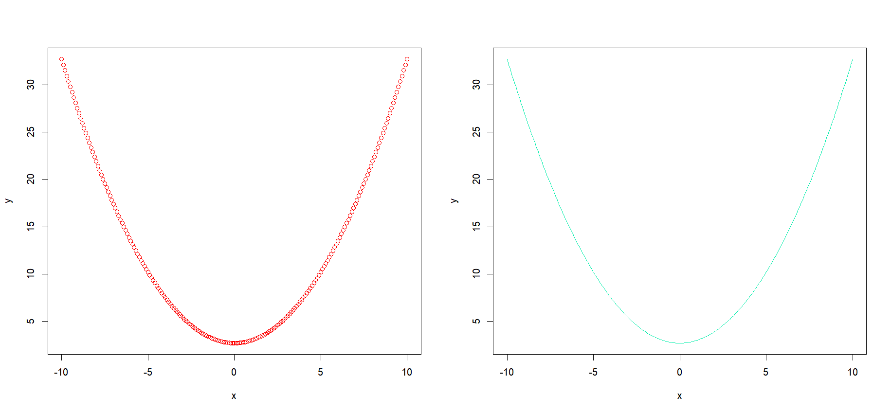
Oh, and if you don’t like the color of your points/lines, you can change it by the argument “col”. The color can be set either by calling it by its name, or through an RGB code:
plot(x,y,type="p",col="red")
plot(x,y,type="l",col="#00EEAA")
Results of the 2 last instructions, side-by-side:
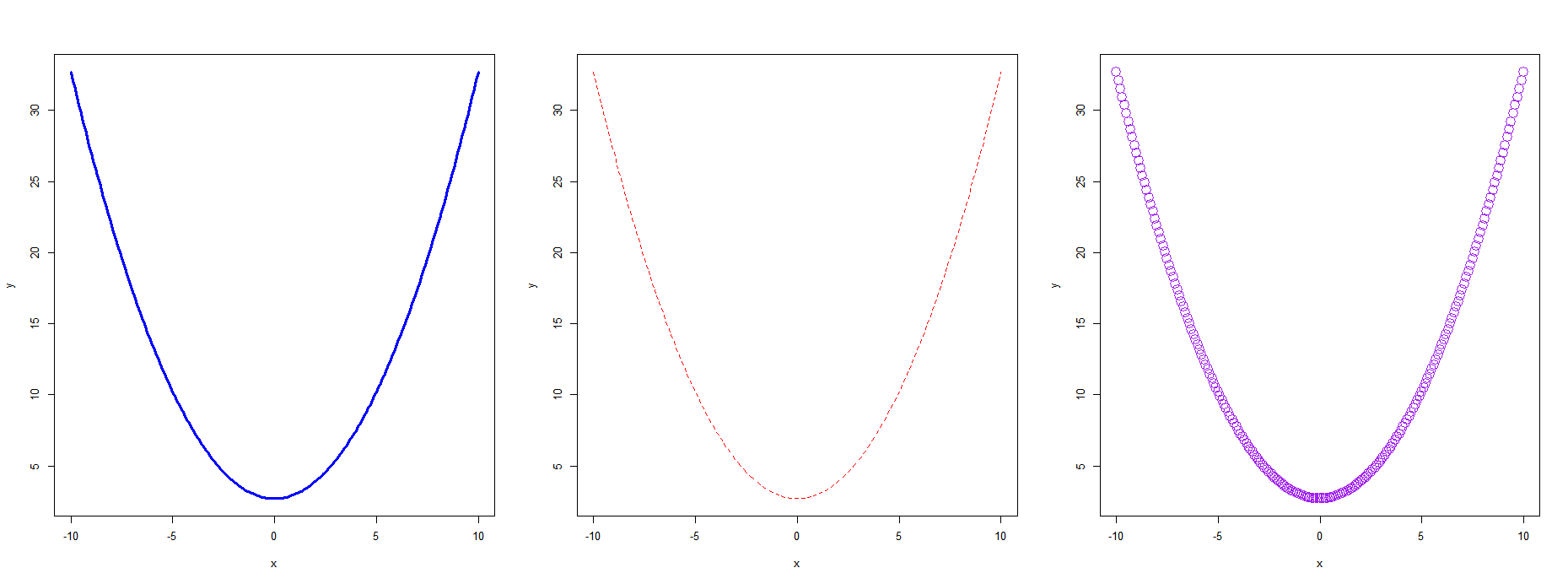
Want a wider/thinner line? You can change the thickness with the argument “lwd” (for line width):
plot(x,y,type="l",col="blue",lwd=3)Fancy a different type of line? You can use dashed lines for example with the argument “lty”. Lines can be one of the following types: “blank”, “solid”, “dashed”, “dotted”, “dotdash”, “longdash”, or “twodash”
plot(x,y,type="l",col="red",lty="dashed")You’re using symbols and they are too big/small? You change modify their size with the argument “cex” (for character expansion)
plot(x,y,type="p",col="purple",cex=2)Results of the last 3 commands:
Pretty nice, isn’t it? But wait… Now that I’m looking at our plot, I just realize that we are missing a title! How could I forget that??? No problem, once again. I can either add a main title (on top), or a subtitle (under the graph) with the arguments “main” and “sub” respectively:
plot(x,y,type="l",col="green",main="So much beauty")
plot(x,y,type="l",col="green",sub="Sneaky!")
plot(x,y,type="l",col="green",main="WOW",sub="At the same time???")
Results of the last 3 commands:

Oh, and since we are talking about text, you can also change the default names for the axis (by default, R takes the name of the plotted variables) with arguments “xlab” and “ylab” for the X-axis and Y-axis respectively:
plot(x,y,type="l",xlab="Nice day, isn't it?",ylab="Why are you guys tilted?")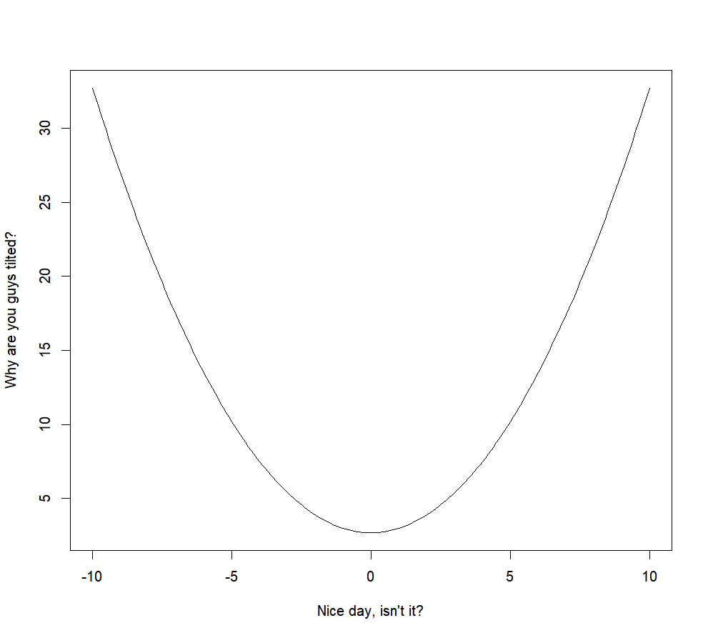
As you can see, all the arguments can be used at the same time, to allow you to totally customize your graph.
A lot (and I mean a LOT) of other options are available, and it would be worth it for you to look at the help for the “par()” function to see all the main elements that can be modified.
Another way of adding titles and axes’ names is to use the function “title()” that will add to the currently active plot those information.
plot(x,y,type="l",xlab="",ylab="")
title(main="A nice smart title", sub="A subtle subtitle", xlab="The treasure marker X-axis", ylab="The questioning Y-axis")
Finally, if you are feeling adventurous, you can also change the shape of the box surrounding the graph (argument “bty”, for box type). The values that this argument can take are: “o” (the default), “l”, “7”, “c”, “u”, or “]” the resulting box resembles the corresponding upper case letter. To suppress the box altogether, you can set it to “n” (for “none”).
plot(x,y,bty="l")
plot(x,y,bty="c")
plot(x,y,bty="n")
will give respectively:
If you want to set some graphical parameters such as the width of your lines, the color of the background, the font of your text, etc… without having to enter those parameters every time, it is possible to use the “par()” function that will set a large number of graphical parameters for the currently active plot window. Every plot that will then be drawn in this window will follow the values set through the function “par()” (unless specified otherwise), and this until said window is closed. It is possible to access the current graphical parameters settings by calling the “par()” function without arguments. This can also be used to save those current parameters in an object.
par()
par.default=par(no.readonly=T)    # Saving current graphical parameters, the argument “no.readonly” allows us to only save the parameters that can be changed
We can then, for example, change the background color, with the argument “bg”, and without a problem subsequently restore the graphical parameters to their defaults values:
par(bg="grey")
plot(x,y,bty="l")
par(par.default)   # resetting the parameters to their default values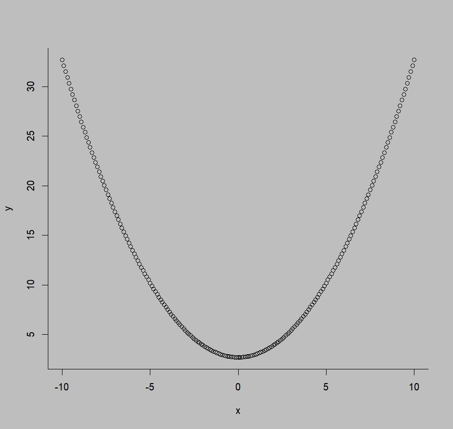
A really interesting feature offered by “par()” is the possibility to open a graphical window where several graphs can be presented at the same time. To do so, we use the argument “mfrow”, and set it through the use of a vector containing two information: the number of rows, and then the number of columns. For example setting “mfrow=c(3,2)” will allow us to plot in the same window 2*3=6 different graphs, with 2 graphs per line over 3 lines. But see for yourself:
par(mfrow=c(3,2))
plot(student~father,main="Student's size depending on father's size")
plot(student~mother,main="Student's size depending on mother's size")
plot(mother~father,main="Wife's size depending on partner's size")
hist(student,breaks=20, main="Students' size frequency")
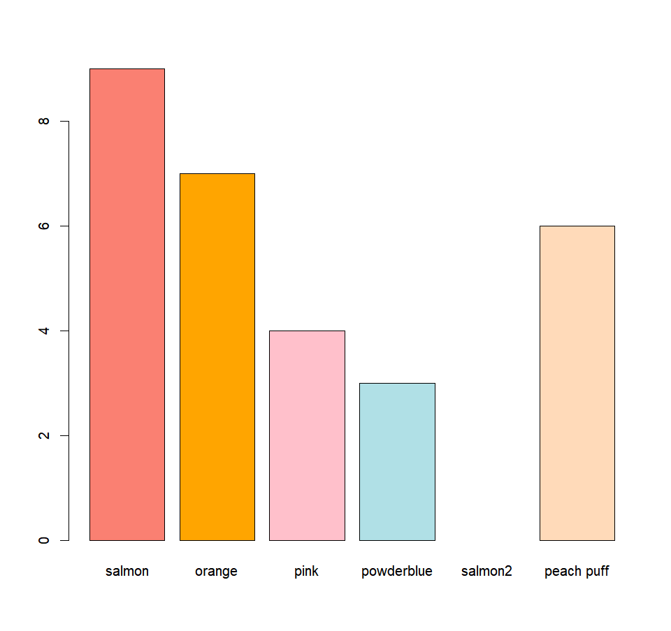
barplot(awesomeness,names=color,col=color,main="Ryan Reynolds's shirts")
plot(x,y,type="l",col="red", main="A nice quadratic curve") 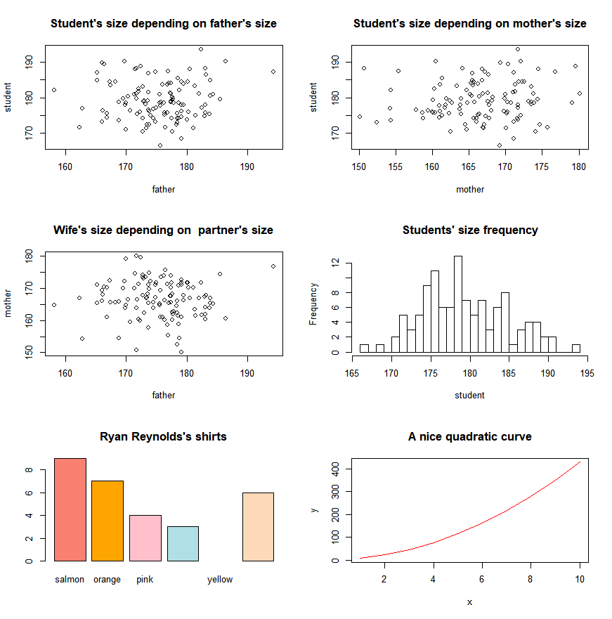
If you need to open a new graphical window, you can do so, either with the function “x11()” or really intuitively with “windows()”
x11()
plot(x,y,type="l",col="blue", main="Here it is again!") 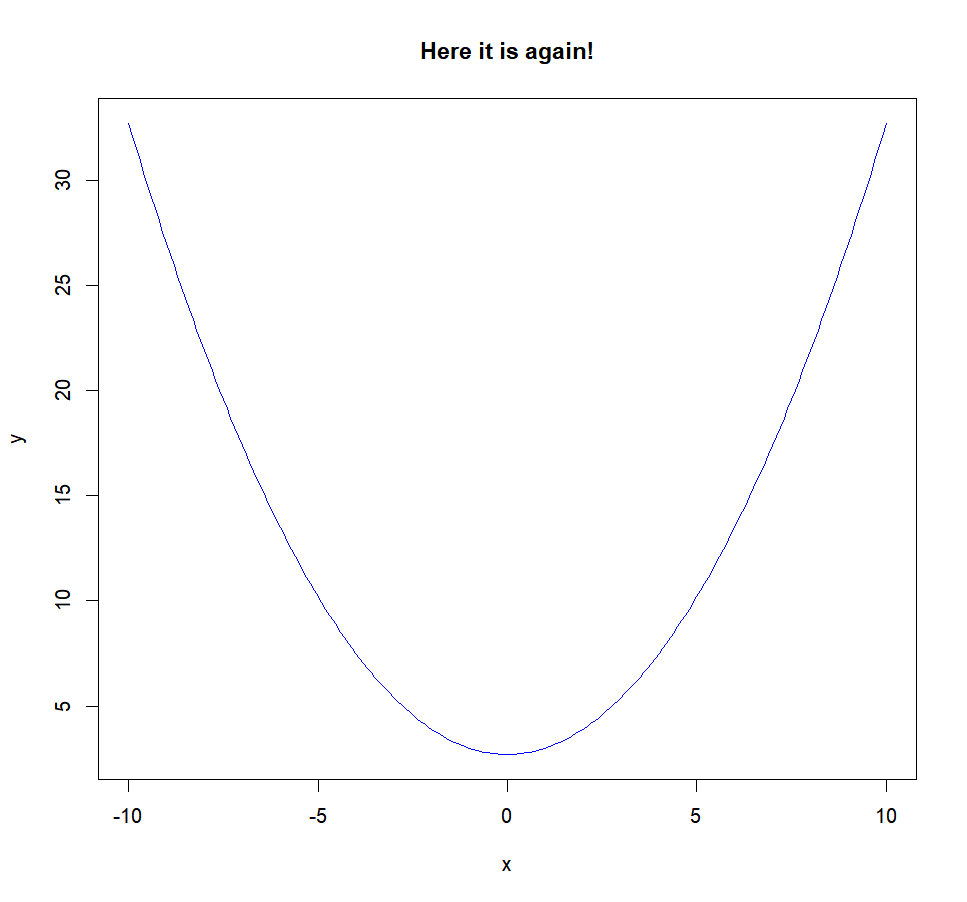
windows()
plot(x,sin(y),type="l",col="green", main="Getting original") 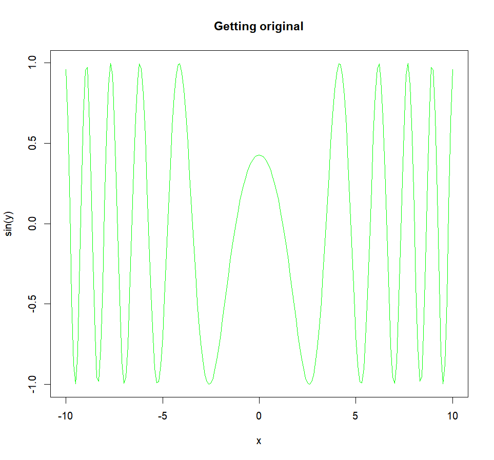
MORE GRAPHICAL FUNCTIONS
Want a histogram? A boxplot? A barplot? You came to the right place!
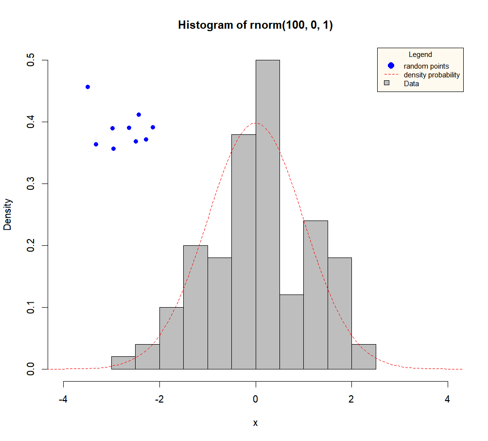
ADDING ELEMENTS
A look at putting finishing touches to your masterpiece.
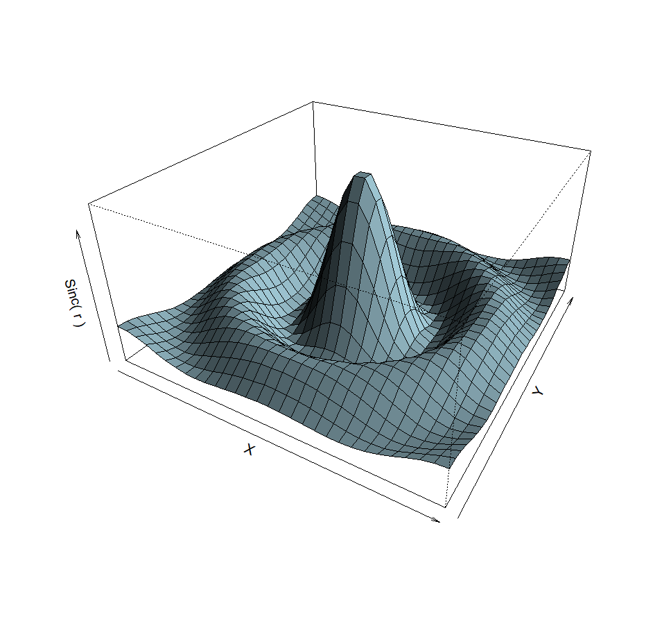
A LITTLE BIT OF 3D?
2D is so 1990. 3D is the future.
GETTING INFORMATION
Or how to interact with your graph!