LET’S TALK ABOUT THE CRUX OF THE MATTER FOR A BIT : DATA!

Crux of the matter: DATA!

R attaches to each object a “class“, this could be seen as a label on the box that indicates the kind of element the “box” (object) contains (is it a number? characters? maybe a matrix?). This in turn allows each function to know what to do when presented with an object. “Can I do anything with what is in this box? Let me look at the label! Our box contains a matrix? Perfect, I know how to deal with that, and what I can do once I open the box to work with what’s inside!”.

We have already seen that we can put things like numbers in our objects. But we can as easily put characters or string of characters (sometimes called “words” in the vernacular), data frames or matrices. But wait, there is more! If you keep reading this in the next 10 min, we also include factors, logical (i.e. True, False, or missing values) and even lists (which for example can be used to put in the same box/object several objects, of possibly different types or classes). You can even create your own class if you ever create functions that need to do particular things when they see some specific type of object. But this is for a slightly more advanced use of R. Let’s take a look at the most common objects we can create and use.

We have already seen that we can create vectors that will contains numbers with the function “c()“, where each element is separated by a comma. If needed, we can leave some of the elements empty, for missing data for example by using NA (for Not Available).

Ok, what about an example of all of that? Shall we create a nice dataset about Ryan Reynolds’ best shirts based on their colors, graded on a scale from 1 to 10?

Characters or strings of characters are indicated between quotes.

color=c("salmon","orange","pink","powderblue","salmon2","peach puff")
awesomeness=c(9,7,4,3,NA,6)  # Yep, the other salmon one (aka salmon2) is too awesome to be rated on our grade. We can't evaluate it.

BTW, if you mix number and characters in a vector, R will interpret all of them as simply character… Needless to say that at this point, without saying anything to R, it will be impossible to do any type of computation on it:

tmp=c(2,"a")
tmp+2
Error in tmp + 2 : non-numeric argument to binary operator
tmp
[1] "2" "a"

Just for fun, we can really easily illustrate our data:

barplot(awesomeness,names=color,col=color)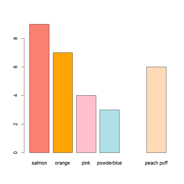

But we’ll see more on plots in the 4th chapter of our R class.

Rather have your data nicely organized in a beautiful data frame? Nothing easier! You can simply use the function “data.frame()“:

shirts=data.frame(color,awesomeness)
shirts
       color awesomeness
1     salmon          9
2     orange          7
3       pink          4
4 powderblue          3
5     yellow         NA
6 peach puff          6

We now have a nicely organize data frame that contains 2 columns, of different classes: first column, the colors (that R smartly, automatically and by default treat as factors), and 2nd column their awesomeness (numerical values). Data frames are used when your data contains elements of different classes in different columns. For example, you could record for Ryan’s shirts: their size, their length, their colors, their price, their awesomeness, and whether or not they match the corresponding shorts; each information contains in a different column. This is generally the type of data we will be dealing with in Ecology.

Conversely, one might have a dataset where all of the rows and columns of a matrix must have the same class (numeric, character, etc). For example, if you are courageous, you could record the length of several bears’ teeth over the years. Each column would correspond to a different year, and each row to a different bear. In this case, you might want to use a matrix. You simply need to specify the corresponding data, and the dimensions of your matrix (number of rows and columns). Example for 3 bears, over 4 years:

bear= matrix(data = c(2.00 , 2.17 , 2.57 , 3.40 ,
                      1.50 , 1.98 , 2.14 , 2.93 ,
                      2.75 , 3.02 , 4.44 , 4.46 ),
             nrow = 3, ncol = 4, byrow=T)

Spaces and lines are here just to make it looks easier to read, but are not necessary for R to understand what you are talking about.

By default, R will fill the matrix starting with the first column, fill all the rows in the first column, then go to the next column and do the same thing, and so on until the table is filled. You can change this by setting the argument “byrow” to “True” or “T” for short. This way R fill all the columns of the first row first, then go to the next one, and so on.

Go on and try it, enter the previous code but with “byrow” set to “False” or “F” for short, and see what happens.

You can similarly create a multidimensional matrix with the function “array()“. To do so, first, specify the data, and then -in a vector- the size of each dimension. For example, while trying to figure out the occupancy of the campus by students, we went on the campus at 3 locations (cafeteria, classes, and library), on 4 different days (Christmas, New Year Eve, mid-terms and December 1). For each day we listened for 2 10-minutes sessions for signs of student presence. Results looked a little bit like that:

  cafeteria=matrix(c(0,0,         # Nobody seen at all during Christmas
                     0,1,         # Student heard during the second session of New-Year Eve
                     1,0,         # Student seen rushing through the hallway during the first session during the mid-terms
                     1,1),        # Students on both sessions on Dec 1
                     nrow=4,ncol=2,byrow=T)
  library = matrix(c(0,0,         # Nobody seen at all during Christmas
                     0,0,         # Not a peep during New-Year Eve
                     1,1,         # Student seen preparing  during the mid-terms
                     1,1),        # Students studying hard seen on both sessions on Dec 1
                     nrow=4,ncol=2,byrow=T)
  classes = matrix(c(0,0,         # Nobody seen at all during Christmas, surprisingly...
                     1,0,         # Student heard during the first session of New-Year Eve, he looked lost...
                     1,1,         # Student seen during both sessions trying to grasp a last bit of wisdom before the exam during the mid-terms
                     1,1),        # Students on both sessions on Dec 1
                     nrow=4,ncol=2,byrow=T)

We can easily keep all that information in one larger dataset, where one dimension corresponds to the day, one to the session, and one to the location.

students <- array(data = c(cafeteria,library,classes),
                  dim=c(4,2,3))

It is, of course, possible to create the array directly by entering the data, without going through the extra step of creating vectors. Moreover, you don’t have to limit yourself to 3 dimensions, if you want to have more, simply specify it accordingly with the “dim” argument.

We can express some of our data as factors. To encode the element of a vector into factors, simply feed the vector to transform to the function “factor()“. For example, if we record the reaction of 6 contestants in a “random” reality TV show where they are subjected to test. We could sort their reactions in 3 categories: “scared”, “courageous”, or “insane”. First, let’s put that information in a vector.

fear=c("scared","scared","courageous","scared","insane","courageous")

But, wait, R recorded each entry in the vector as a string of character.

class(fear)   # The function "class()" allows us to display the current class of an object
[1] "character"

Some analyses (like glm’s) will want to work with factors, rather than with simple characters. Let’s convert our vector:

fear=factor(fear)
class(fear)
[1] "factor"

We can also easily access the different levels used as factors in our vector with the function “levels()“.

levels(fear)
[1] "courageous" "insane"     "scared"

Now, while in general factors do not refer to numbers, they may in certain cases. This might be the source of confusion. If you try to directly transform your levels back into a number, something funny will appear…

numfac=factor(c(101,102,103))
numfac
[1] 101 102 103
Levels: 101 102 103

as.numeric(numfac)  # Trying to convert our vector back to numbers
[1] 1 2 3

What happened? R is returning “1 2 3”!!! That’s not what we put as numbers in! Indeed, we did! But when R converted our numerical vector to a factor vector, it stopped considering those as numbers. Instead, it replaced each element with a level. The first level is assigned the number 1, the 2nd the number 2, etc. In our case, R took ‘101’ and assigned it the level 1. It keeps in memory that the level 1 is called ‘101’, but that’s it. If your factor represents numbers and you want to recover those numbers from the factor, then you need a little bit of extra work. One way of doing it is to first convert your factors as characters, and then finally as number.

 

as.numeric(as.character(factor(101:103)))
[1] 101 102 103

Yep… Dealing with factors can be slightly counter-intuitive…

The last type of data we are going to discuss today: lists. Lists are generic vectors containing other objects in an ordered manner. A big box containing several different boxes. A list is an ordered collection of objects, and therefore allows you to gather a variety of (possibly unrelated) objects under one name.

data=list(shirts=shirts,students=students,somerawdata=color)

My “data” object now contains three objects: a dataframe (shirts), an array (students) and a vector (color, that I’ve conveniently renamed as “somerawdata” in my list object!).