COMPARING MORE THAN TWO SAMPLES: SINGLE FACTOR ANALYSIS OF VARIANCE

Comparing more than two samples: single factor analysis of variance

Let’s assume that you like life to be complicated, that you are ambitious and that you don’t think you should limit yourself to studying only two samples. First, congrats, aim for the moon, if you fail, I’m sure that there is cheese somewhere else! Second, as always, I’m here to help.

We can in this case perform an ANOVA (ANalysis Of VAriance). Several functions are available in R to do this test, and I’ll focus here on the function “aov()“, because why not! As for Student’s t-test, the ANOVA makes some assumptions: your samples should be independent, assumed to have the same variance, and the residuals should be normally distributed (with a mean 0); if it’s not the case and you are dealing with a small sample size, go check the next section.

The ANOVA will tell you if at least one of your samples has a mean that is different from the two others. If it’s the case, you will still need to determine which sample(s) is responsible for this with a multiple comparison test like the Tukey Honest Significant Difference (HSD) test (also known as Tukey’s range test).

Let’s take a quick example. First, we need data… I’ve compiled ratings for movies’ awesomeness with actors Sylvester Stallone (“SS”), Arnold Schwarzenegger (“AS”), Bruce Willis (“BW”) and Jean-Claude Van Damme (“JCVD”). Each actor has several movies; each movie has its own rating.

Entering the data:

actor=c("SS", "JCVD", "JCVD", "BW", "SS", "JCVD", "SS",
        "BW", "BW", "SS", "BW", "JCVD", "JCVD", "JCVD", 
        "AS", "AS", "BW", "BW", "AS",
        "AS", "JCVD", "BW", "AS", "SS", 
        "SS", "BW", "AS", "BW", "JCVD", "AS",
        "SS", "JCVD", "AS", "SS")
rating=c(2.27, 1.25, 1.15, 1.62, 1.7, 0.63, 2.05, 2.19, 2.1, 2.2, 2.06, 
 1.9, 1.88, 0.85, 1.83, 1.88, 2.02, 1.94, 2.1, 2.38, 1.43, 1.75, 
 2.83, 1.53, 0.76, 0.8, 1.66, 0.98, 1.04, 2.18, 1.89, 1.37, 1.4, 
 1.98)

Putting it in a data.frame, because it’s nicer and it’s what the function “aov()” needs.

film=data.frame(actor,rating)
View(film)

With the function “tapply()“, we can calculate the “mean” of the “rating”s depending on the “actor” in our “film” data:

tapply(film$rating, film$actor, mean)
      AS       BW     JCVD       SS 
2.032500 1.717778 1.277778 1.797500

The actual analysis is performed by specifying to the function which response variable is changing in function of which factor(s), followed by the name of the data frame where the data are. In our case, we are interested by how films’ ratings are influenced by the lead actor. This is simply given to R with the formula “rating~actor”.

aov.res=aov(rating~actor,data=film)
summary(aov.res)
            Df Sum Sq Mean Sq F value Pr(>F)  
actor        3  2.567  0.8555   3.939 0.0176 *
Residuals   30  6.516  0.2172                 
---
Signif. codes:  0 ‘***’ 0.001 ‘**’ 0.01 ‘*’ 0.05 ‘.’ 0.1 ‘ ’ 1

In the summary, we can see that at least one of the groups is different from one other group, as established through the factor “actor”. Or: the variable “actors” has an effect on the response variable “rating”. In our case, it means that at least one of the actors has on average better ratings than at least one of the other actors.

For the most observant of you, you’ll notice that at this stage, we have no idea who is whom! We’ll figure that out in a moment with a multiple comparison test: the Tukey HSD test. But before that, we’ll make sure that our 2 primary assumptions are met: same variances (also called homoskedasticity) and residuals normally distributed.

Let’s check the normal distribution of our residuals. First, we need to access the residuals. They are available in the results provided by the function “aov()”, life is well done, right?

aov.res$residuals
     1         2           3           4           5           6           7
 0.472500 -0.027777 -0.127777  -0.097777   -0.097500   >-0.647777    0.252500
     8         9          10          11          12          13          14
 0.472222  0.382222  0.402500    0.342222    0.622222    0.602222   -0.427778
    15         16          17          18          19          20          21
-0.202500 -0.152500  0.302222    0.222222     0.067500    0.347500   0.152222
    22         23          24          25          26          27          28
 0.032222  0.797500 -0.267500   -1.037500    -0.917778    -0.372500 -0.737778
    29         30          31          32          33          34
-0.237778  0.147500  0.092500     0.092222   -0.632500   0.182500

Now that we know where the residuals have been saved, we can look at them and see if they have a normal distribution. To do so, we’ll plot a Q-Q (quantile-quantile) plot which will show us the actual residuals quantiles plotted against theoretical normal quantiles. If our residuals are normally distributed, they should fall neatly along a line that corresponds to a “theoretical” normal quantile-quantile plot.

Plotting our residuals’ quantiles:

qqnorm(aov.res$residuals)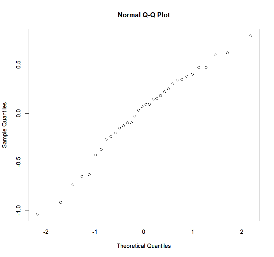

Adding the line indicating normality:

qqline(aov.res$residuals)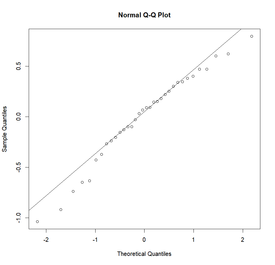

In our case, it looks pretty good. But to be sure, and not simply rely on our guts, we can use the Shapiro test:

shapiro.test(aov.res$residuals)
        Shapiro-Wilk normality test
data:  aov.res$residuals

W = 0.9688, p-value = 0.43

Here, p is higher than 0.05, therefore we can reject H1 (“Residuals are not normally distributed”), or more exactly, we cannot reject H0 (“Residuals are normally distributed”).

Then, we can test for homogeneity of variances with a Bartlett test, following the same syntax as with the function “aov()”:

bartlett.test(rating~actor,data=film)
        Bartlett test of homogeneity of variances
data:  rating by actor
Bartlett's K-squared = 0.2529, df = 3, p-value = 0.9686

Same thing here, the corresponding probability is higher than 0.05, therefore we cannot reject H0 (“Variances of our different groups are equal”).

Therefore, our assumptions were met, and we’re clear to proceed to the next step: determining which group(s) is/are different from the others. To do that, we’ll perform a Tukey HSD test. This test will compare two by two the different groups and determine which are significantly different from the others. To do this test, we simply input the object containing the results from the ANOVA to the “TukeyHSD()” function.

TukeyHSD(aov.res)
  Tukey multiple comparisons of means
    95% family-wise confidence level
Fit: aov(formula = rating ~ actor, data = film)
$actor
               diff         lwr        upr     p adj
BW-AS   -0.31472222 -0.93050636  0.3010619 0.5153456
JCVD-AS -0.75472222 -1.37050636 -0.1389381 0.0116543
SS-AS   -0.23500000 -0.86863665  0.3986367 0.7457444
JCVD-BW -0.44000000 -1.03739837  0.1573984 0.2095597
SS-BW    0.07972222 -0.53606192  0.6955064 0.9847376
SS-JCVD  0.51972222 -0.09606192  1.1355064 0.1218677

Here, the only statistically significant difference is observed between the movies with JCVD and AS, where JCVD on average has worse movies than AS.

We can graphically represent those results by plotting the results of our Tukey HSD test:

plot(TukeyHSD(aov.res))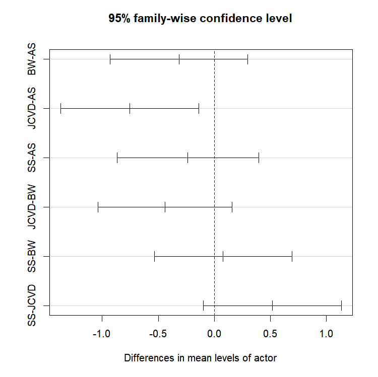

The only 95% confidence interval that does not include 0 is the one representing the comparison of the ratings for the movies of AS and JCVD!

Properly realizing an ANOVA has never been easier.

testA=rnorm(50,135,20)
testB=rnorm(37,154,15)
t.test(testA, testB, var.equal=F)
testC=rnorm(42,143,12)
fac=c(rep("A",50),rep("B",37),rep("C",42))
vec.all=c(testA,testB,testC)
data.test=data.frame(vec.all,fac)
aov.res=aov(vec.all~fac,data=data.test)
summary(aov.res)
qqnorm(aov.res$residuals)
qqline(aov.res$residuals)
shapiro.test(aov.res$residuals)
bartlett.test(vec.all~fac,data=data.test)
TukeyHSD(aov.res)
plot(TukeyHSD(aov.res))