Regression between two variables
Determining the slope linking two variables: the simple linear regression
Now that we know how to estimate the strength of a relationship between two variables, we can try to define this relationship.
The simple linear regression is used when trying to find the relationship between a continuous response variable and one explanatory variable. Let’s try to fit a linear model for those data with the function “lm()“, by specifying the expected relationship between the two variables with a formula Y~X, and letting the function know where the data are.
Example time
A certain individual named Walter White is trying to figure out the relationship between the purity of his product, and the price people are willing to pay for it:
profit=data.frame(purity=c(4.5,9,22.5,45,90),price=c(22.45,66.81,209.19,508.06,998.13))
profit
  purity  price
1    4.5  22.45
2    9.0  66.81
3   22.5 209.19
4   45.0 508.06
5   90.0 998.13
For the regression:
results=lm(price~purity,data=profit)  # we are storing the results in an object named "results" (because we're smart)
summary(results)    # we ask for a summary of the results (because we're curious)
Call:
lm(formula = price ~ purity, data = profit)
Residuals:
      1       2       3       4       5
  4.381  -3.207 -16.672  22.456  -6.958
Coefficients:
            Estimate Std. Error t value Pr(>|t|)
(Intercept) -33.8799    11.2249  -3.018   0.0568 .
purity       11.5441     0.2423  47.648 2.04e-05 ***
 ---
Signif. codes:  0 ‘***’ 0.001 ‘**’ 0.01 ‘*’ 0.05 ‘.’ 0.1 ‘ ’ 1
Residual standard error: 16.93 on 3 degrees of freedom
Multiple R-squared:  0.9987,    Adjusted R-squared:  0.9982
F-statistic:  2270 on 1 and 3 DF,  p-value: 2.035e-05
A little help to interpret the results?
First, R is reminding us about what we asked him to do. Then, the residuals. Residuals correspond to the distance left between our data points and the regression line. If residuals are systematically positive, then negative (or the other way around), it means that our data are probably not linear. The relationship between our 2 variables might be better explained by a curve for example (but a look at the raw data should have already raised some suspicion). No real problem in our case. The rest of the table can be analyzed as the results of an ANOVA. Here, the intercept is not significantly different from 0 (p=0.057). It could be interpreted as: for a purity of 0, nobody would be willing to pay anything for Heisenberg… erm, sorry… for Walt’s product. The purity effect is statistically highly significant (p<0.001). This would attest a causal relationship: the purer the product, the more expensive it can be.
We could then write this relationship as:
| price=11.54*purity – 33.88′ |
Oh, and by the way, noticed that our table also returns the coefficient of determination? Here, 0.9987.
Before going further, I have a request: do me a favor and don’t blindly accept the results of a linear regression. While the summary provided is certainly interesting, as it is right now, it’s missing elements that will allow us to evaluate the model’s suitability at explaining our data. The easiest way of doing so is to visually examine the residuals. To determine if the model is appropriate, it has to meet certain criteria such as:
- the residual errors should be random and normally distributed,
- removing one case should not significantly impact the model’s suitability.
R provides four graphical approaches to evaluate a model by plotting the linear regression results:
plot(results)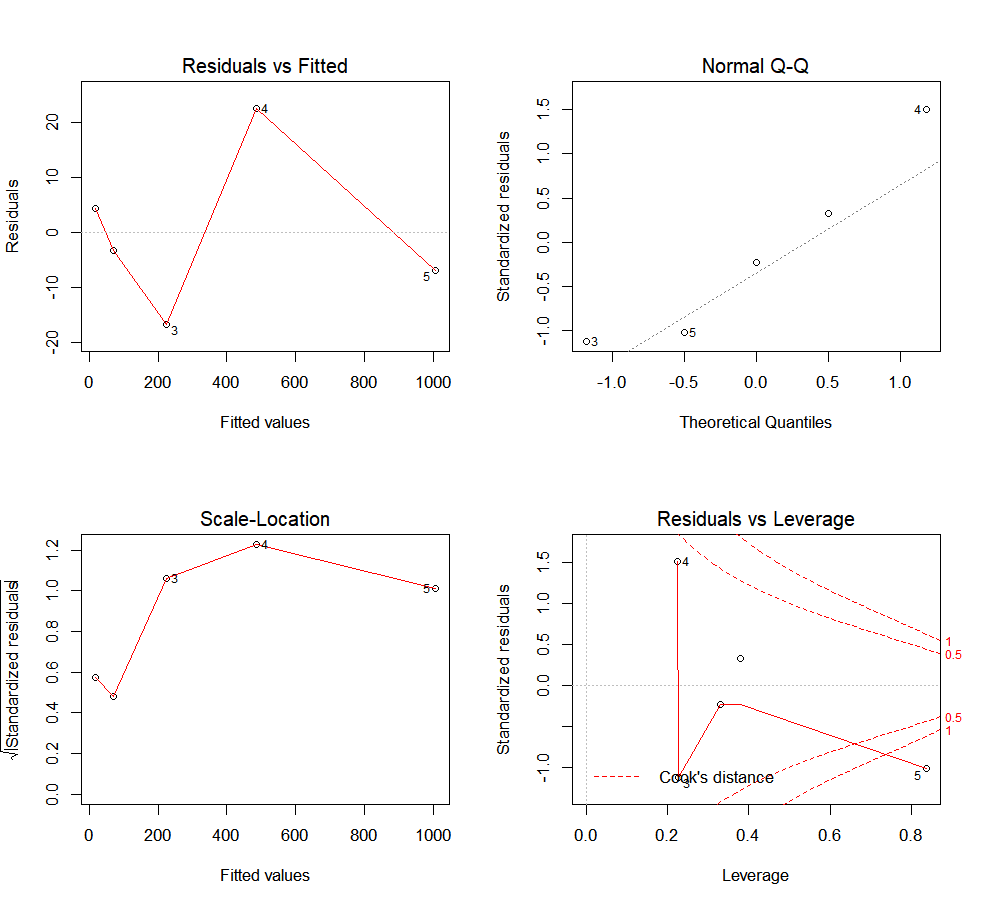
The first plot (top-left) shows the residual errors plotted against the fitted values. The residuals should be randomly distributed around the horizontal line. No distinct trend or pattern should be visible in this graph. A graph presenting points that follow a curve or a trend instead of the horizontal line would be indicative of non-linear or biased residuals. A conic points cloud would indicate heteroskedasticity (feel free to use this word when playing Scrabble, it always impresses people). Simply put, variance would not be constant over the data range (it could for example increase as the explanatory variable increases. Both of those are indications that the model is not adapted to our data. On a side note, you might have noticed that this plot is simply a rotation of the plot “y in function of x”, so that the linear regression line is horizontal.
The second plot (top-right) is a standard Q-Q plot. As we have seen with the ANOVA, it allows us to check that residual errors are normally distributed. If it is the case, they should follow the diagonal line indicating normality.
The third plot (lower-left) is called a scale-location plot. It shows the square root of the standardized residuals as a function of the fitted values. Once again, if your model is suitable, you should not detect any obvious trend in this plot.
And finally, the fourth plot (lower-right) will represent each point’s leverage. The higher the leverage, the more important the corresponding point is in determining the regression coefficient/results. Superimposed on the plot are contour lines for the Cook’s distance. This presents another measure of the importance of each observation to the regression. A smaller distance means that removing the corresponding observation would not impact regression results. However, distances larger than 1 are suspicious and could indicate that the presence of an outlier or that we have a poor model.
Moreover, as you might have noticed, R is even nice enough to label the data points that might require further examination with their indices.
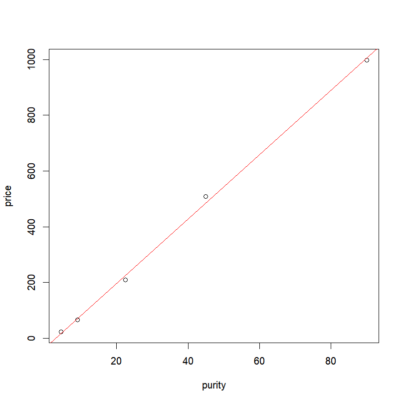
In the case of a simple linear model with one covariate, it is really easy to plot those results. First we plot our points:
plot(price ~ purity, data = profit) Then, we just need to add the fitted line from the object containing the linear regression results:
abline(results, col="red" )or
abline(lm(price~purity,data=profit), col="red" )Final result:
Another more versatile option is to predict values based on our model (this can be used with more than one variable). In order to predict the values, we need a) the results of the model we used, b) a data frame (for the argument ‘new.data’). Each column of the data frame must contain the values of the explanatory variables for which we are trying to predict the response variable. And c) we need to feed the “predict()” function with aforementioned model results and predictive variables.
Step a)
lm.results <- lm(price ~ purity, data = profit)Step b)
Here, we simply want to predict values over the range of our explanatory variable, with a data frame with a single explanatory variable. Important note: the name of the created explanatory variable in the data frame has to be the same as the original one used in the model.
xnew <- seq(min(profit$purity), max(profit$purity),
            length.out = 100)
expl.pred=data.frame(purity = xnew)
The function “seq(A,B, length.out =N)” creates a vector containing a sequence of N values ranging from A to B, but more on that later.
Step c)
We then feed the model, and the data frame containing the explanatory variable (‘purity’) values over which we want to predict our response variable (‘profit’). We can even ask for the 95% confidence interval by setting ‘interval = “confidence” ‘ and ‘level = 0.95’
resp.pred <- predict(lm.results, newdata= expl.pred,
                     interval = "confidence", level = 0.95)
resp.pred <- data.frame(resp.pred)                  # Conversion to a data frame so the values can easily be accessed by the plotting functions
The fitted values are contained in the column ‘fit’ of our “predict()” output. The lower and upper confidence intervals are contained in the columns ‘lwr’ and ‘upr’ of our “predict()” output.
We just have to plot the data, add the fitted line, and the confidence intervals with the function “lines()”.
plot(price ~ purity, data = profit)
lines(resp.pred$fit ~ expl.pred$purity,col="red")      # Fitted values
lines(resp.pred$lwr ~ expl.pred$purity, lty = "dashed")# Lower 95% interval
lines(resp.pred$upr ~ expl.pred$purity, lty = "dashed")# Upper 95% interval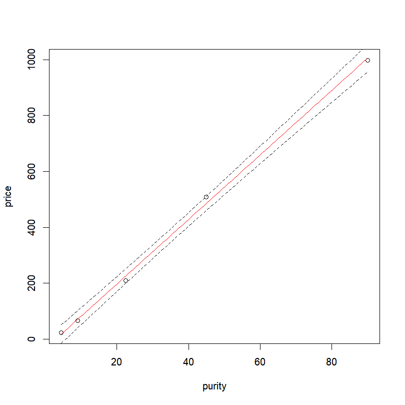
The arguments “col” and “lty” allow us to specify the line color and type respectively (here red for the fitted values and dashed for the confidence interval). Final result:
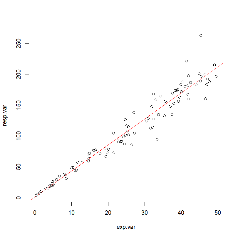
Exercise 3.3– Create a vector ‘exp.var’ of 100 values following a uniform distribution ranging from 0 to 50 – Create a vector ‘slope.var’ of 100 values following a normal distribution with a mean of 4.3 and a standard deviation of 0.5 – Create a vector ‘inter.var’ of 100 values following a normal distribution with a mean of 2.7 and a standard deviation of 0.2 – Create a vector ‘resp.var’ equal to the product of ‘exp.var’ and ‘slope.var’ plus ‘inter.var’ – Plot ‘resp.var’ against ‘exp.var’ – Calculate and test the correlation between ‘resp.var’ and ‘exp.var’ – Compute the regression analysis modeling ‘resp.var’ in function of ‘exp.var’ – Plot the results of the regression analysis< – Plot the regression line over the data
|
Determining the slope linking more than two variables: the multiple linear regression
We do not need to limit ourselves to 2 variables (1 response vs 1 explanatory). It is frequent in ecological studies to consider the potential relationship between the parameter of interest (such as abundance) and multiple covariates (e.g. precipitations, temperatures, density). Linear models can be used to model the relationship between a continuous response/dependent variable and several explanatory variables. This approach can however only deal with a linear combination of said explanatory variables. That’s why it’s called a linear model.
But what does it mean “a linear combination”? Good question! Holy Darwin, you are insightful! Remember the slope we calculated earlier? For each covariate you are considering, you are estimating a slope coefficient. The imperative of linear combination applies to those coefficients (and not the explanatory variables themselves). It means that slopes are not “interacting” with each other, they affect the response variable in an additive way in regard to each other. Assuming that everything else in the model stays the same, a change by one unit of a covariate (or of any resulting transformation of said covariate) will be reflected by an increase of the response variable equal to the corresponding coefficient.
I apologize for the next lines, but I will need to use some equations to make my point… I promise, I’ll do my best to keep it simple. Ok, so what is a line? A line can be described with the equation “y=ax+c” (where ‘y’ is the response variable, ‘x’ the explanatory variable, ‘a’ the slope coefficient, and ‘c’ a constant). So far, so good, nothing new under the sky. If ‘x’ varies by one, ‘y’ will vary by ‘a’.
Ok, so what is a linear model? The same thing, with potentially more explanatory variables. For example, I could have ‘x1’ and ‘x2’. My equation would become “y=ax1+bx2+c”. If I don’t touch to ‘x2’, then, when ‘x1’ will vary by one unit, ‘y’ still varies by ‘a’. If you were as perceptive as you have been so far, you will remember that I said a little bit earlier that we could use transformation of said covariate. Therefore, “y=ax+bx^2+c” is still a linear model. If you add 1 to ‘x’ while keeping every else constant (even x^2), you still increase ‘y’ by ‘a’. If I wanted to nit-pick, I could replace ‘x^2’ by a dummy variable ‘X’, and the model would become: “y=ax+bX+c”. It should be obvious now that we are dealing with a linear combination of our covariates ‘x’ and ‘X’. This also implies that the plotted result does not need to be a line! As you can see, you can use for example a linear combination of polynomial components, or transform them in an arbitrary way.
So, how do you specify a model with several components? Easy, by “adding” them with a ‘+’ sign.
x1=c(1,2,3,4,5,6,7,8,9,10)
x2=rnorm(length(x1),5,4)
y=4*x1 + 3*x2 + 5 + rnorm(length(x1),0,1)
# 'y' is a function of 'x1', 'x2' with an intercept of 5.
# And we add some noise for good measure.
summary(lm(y~x1+x2))
Call:
lm(formula = y ~ x1 + x2)
Residuals:
    Min      1Q  Median      3Q     Max
-1.1910 -0.4382 -0.1771  0.7388  1.2355
Coefficients:
            Estimate Std. Error t value Pr(>|t|)
(Intercept)   5.2895     0.8110   6.522 0.000327 ***
x1            4.0713     0.1100  37.006 2.74e-09 ***
x2            2.8825     0.1093  26.372 2.89e-08 ***
---
Signif. codes:  0 ‘***’ 0.001 ‘**’ 0.01 ‘*’ 0.05 ‘.’ 0.1 ‘ ’ 1
Residual standard error: 0.9938 on 7 degrees of freedom
Multiple R-squared:  0.997,     Adjusted R-squared:  0.9961
F-statistic:  1147 on 2 and 7 DF,  p-value: 1.551e-09
Results that describe accurately what we were expecting (or more exactly, what we have in our data). One warning: it is essential to not use covariates that are “highly” correlated with each other. If the covariates are highly correlated, the coefficients for each covariate will no longer be able to vary independently, and as you can imagine, it will become “difficult” to obtain 2 separate estimates. One covariate will effectively hide the other.
Similarly, we can remove a parameter from the model by using the sign ‘-‘. For example, if we want to remove the intercept from our model, we can use the instruction ‘-1’ (‘1’ corresponds to “intercept”, and is included in every model unless otherwise specified).
y=4*x1 + 3*x2With intercept:
summary(lm(y~x1+x2))
Call:
lm(formula = y ~ x1 + x2)
Residuals:
       Min         1Q     Median         3Q        Max
-5.380e-15 -4.243e-16  5.388e-16  1.042e-15  3.618e-15
Coefficients:
             Estimate Std. Error   t value Pr(>|t|)
(Intercept) 8.988e-15  2.412e-15 3.726e+00  0.00739 **
x1          4.000e+00  3.272e-16 1.223e+16  < 2e-16 ***
x2          3.000e+00  3.250e-16 9.230e+15  < 2e-16 ***
---
Signif. codes:  0 ‘***’ 0.001 ‘**’ 0.01 ‘*’ 0.05 ‘.’ 0.1 ‘ ’ 1
Residual standard error: 2.955e-15 on 7 degrees of freedom
Multiple R-squared:      1,     Adjusted R-squared:      1
F-statistic: 1.306e+32 on 2 and 7 DF,  p-value: < 2.2e-16
Without intercept:
summary(lm(y~x1+x2-1))
Call:
lm(formula = y ~ x1 + x2 - 1)
Residuals:
       Min         1Q     Median         3Q        Max
-3.673e-14 -4.005e-15  1.403e-15  2.998e-15  8.022e-15
Coefficients:
    Estimate Std. Error   t value Pr(>|t|)
x1 4.000e+00  1.119e-15 3.574e+15   <2e-16 ***
x2 3.000e+00  1.270e-15 2.362e+15   <2e-16 ***
---
Signif. codes:  0 ‘***’ 0.001 ‘**’ 0.01 ‘*’ 0.05 ‘.’ 0.1 ‘ ’ 1
Residual standard error: 1.38e-14 on 8 degrees of freedom
Multiple R-squared:      1,     Adjusted R-squared:      1
F-statistic: 3.988e+31 on 2 and 8 DF,  p-value: < 2.2e-16
While this might not appear important here, this can become interesting to use when using factors, as -by default- the first factor class will be equal use as the intercept.
If you work with ecological questions, you will want to consider possible interactions between covariates. For example, let’s look at the sweetness of my tea in function of the amount of honey I put in it, and the number of times I stir it. If I stir my tea without honey, it’s not going to change how sweet it is. If I put honey without stirring, the tea is not going to taste much sweeter. BUT, if I put honey and stir, the tea is going to become increasingly sweeter. There is an interaction between the amount of honey and the stirring. In order to consider the interaction between those 2 variables, we use the sign ‘:’ between the 2 covariates.
honey=c(0, 0.5, 1, 1.5, 2, 2.5, 3, 3.5, 4, 4.5, 5)
stir=c(1,2,3,4,5,6,7,8,9,10,11)
sweetness= 0.1*honey + 0*stir + 2*honey*stir + rnorm(length(honey),0,1)
Sweetness in function of honey and stirring, but without considering the interaction:
summary(lm(sweetness~honey+stir))
Call:
lm(formula = sweetness ~ honey + stir)
Residuals:
    Min      1Q  Median      3Q     Max
-10.076  -7.430  -1.638   6.256  15.174
Coefficients: (1 not defined because of singularities)
            Estimate Std. Error t value Pr(>|t|)
(Intercept)  -15.250      5.564  -2.741   0.0228 *
honey         22.200      1.881  11.802 8.87e-07 ***
stir              NA         NA      NA       NA
---
Signif. codes:  0 ‘***’ 0.001 ‘**’ 0.01 ‘*’ 0.05 ‘.’ 0.1 ‘ ’ 1
Residual standard error: 9.864 on 9 degrees of freedom
Multiple R-squared:  0.9393,    Adjusted R-squared:  0.9326
F-statistic: 139.3 on 1 and 9 DF,  p-value: 8.873e-07
Noticed how the model can’t compute a coefficient for the “stir” factor? Well, it is not surprising since this factor is by itself not responsible for any variation in our response variable. On the other hand, we manage to detect a link between the honey and the sweetness, but it doesn’t make any sense based on what we defined. If we were to make inferences based on that, we would be totally wrong.
Now, if we consider the interaction:
summary(lm(sweetness~honey + stir + honey:stir))
Call:
lm(formula = sweetness ~ honey * stir)
Residuals:
     Min       1Q   Median       3Q      Max
-1.00410 -0.33325 -0.03291  0.28196  1.37853
Coefficients: (1 not defined because of singularities)
            Estimate Std. Error t value Pr(>|t|)
(Intercept) -0.13012    0.53657  -0.243    0.814
honey        0.02387    0.54576   0.044    0.966
stir              NA         NA      NA       NA
honey:stir   2.01601    0.04809  41.922 1.15e-10 ***
---
Signif. codes:  0 ‘***’ 0.001 ‘**’ 0.01 ‘*’ 0.05 ‘.’ 0.1 ‘ ’ 1
Residual standard error: 0.7043 on 8 degrees of freedom
Multiple R-squared:  0.9997,    Adjusted R-squared:  0.9997
F-statistic: 1.454e+04 on 2 and 8 DF,  p-value: 5.721e-15
Much better! By the way, instead of writing this long equation saying “take my first factor, AND take my second factor AND take the INTERACTION between them”, we can use the sign ‘*’. This way, we are specifying all of the above directly:
summary(lm(sweetness~honey*stir))
Call:
lm(formula = sweetness ~ honey * stir)
Residuals:
     Min       1Q   Median       3Q      Max
-1.00410 -0.33325 -0.03291  0.28196  1.37853
Coefficients: (1 not defined because of singularities)
            Estimate Std. Error t value Pr(>|t|)
(Intercept) -0.13012    0.53657  -0.243    0.814
honey        0.02387    0.54576   0.044    0.966
stir              NA         NA      NA       NA
honey:stir   2.01601    0.04809  41.922 1.15e-10 ***
---
Signif. codes:  0 ‘***’ 0.001 ‘**’ 0.01 ‘*’ 0.05 ‘.’ 0.1 ‘ ’ 1
Residual standard error: 0.7043 on 8 degrees of freedom
Multiple R-squared:  0.9997,    Adjusted R-squared:  0.9997
F-statistic: 1.454e+04 on 2 and 8 DF,  p-value: 5.721e-15
In this case, the multiplication is not considered in its mathematical meaning. If you want to use a mathematical operation with its mathematical meaning instead of its “model specification meaning”, you have to input the corresponding element with the function ‘I()‘. For example:
x=c(1,2,3,4,5,6,7,8,9,10)
y=3*x + 4*x^2
Let’s see what happens if we simply model ‘y’ in function of ‘x’.
summary(lm(y~x))
Call:
lm(formula = y ~ x)
Residuals:
   Min     1Q Median     3Q    Max
   -32    -24     -8     16     48
Coefficients:
            Estimate Std. Error t value Pr(>|t|)
(Intercept)  -88.000     22.199  -3.964  0.00415 **
x             47.000      3.578  13.137 1.07e-06 ***
---
Signif. codes:  0 ‘***’ 0.001 ‘**’ 0.01 ‘*’ 0.05 ‘.’ 0.1 ‘ ’ 1
Residual standard error: 32.5 on 8 degrees of freedom
Multiple R-squared:  0.9557,    Adjusted R-squared:  0.9502
F-statistic: 172.6 on 1 and 8 DF,  p-value: 1.073e-06
Doesn’t really make sense. Let’s include the quadratic component on top of the linear component:
summary(lm(y~I(x*x)+x))
Call:
lm(formula = y ~ I(x * x) + x)
Residuals:
       Min         1Q     Median         3Q        Max
-9.142e-14 -1.872e-14 -9.265e-15  2.129e-14  1.067e-13
Coefficients:
              Estimate Std. Error    t value Pr(>|t|)
(Intercept) -1.258e-13  6.694e-14 -1.880e+00    0.102
I(x * x)     4.000e+00  2.477e-15  1.615e+15   <2e-16 ***
x            3.000e+00  2.796e-14  1.073e+14   <2e-16 ***
---
Signif. codes:  0 ‘***’ 0.001 ‘**’ 0.01 ‘*’ 0.05 ‘.’ 0.1 ‘ ’ 1
Residual standard error: 5.692e-14 on 7 degrees of freedom
Multiple R-squared:      1,     Adjusted R-squared:      1
F-statistic: 2.943e+31 on 2 and 7 DF,  p-value: < 2.2e-16
We get what we were expecting. Without the function “I()”, R would have read this as “y in function of x and the interaction between x and x”.o