Function: in the loop
The goal of a function is often to make our life easier when repetitive and/or complex operations have to be done. One way of doing that in R is through loops.
“for() {}”: the loop of it!
The most versatile kind of loop is specified with the instruction “for (A in B) { f(A) } “.The instructions ‘f(A)‘ between brackets will be repeated for each element ‘A‘ within the vector ‘B‘. I’m pretty sure that the last sentence is not perfectly clear, so let’s try to explain that differently. The instructions to be repeated (between brackets) will involve a variable. This variable is contained in a vector specified after the word “in”. The variable is assigned in turn the value of each element of the vector, and referred to in the subsequent code in brackets by the name specified as ‘A’. Let’s take an example to illustrate that.
# I'm going to alternatively assign each value contained
# in the vector  c(2,1,...,40) to an object called "variable"
for (variable in c(2,1,6,5,9,40) ) {
    # After assigning each element from the vector to "variable",
    # I'm going to perform the instruction between brackets.
    # Here, displaying said element.
    print(variable)
    }
[1] 2
[1] 1
[1] 6
[1] 5
[1] 9
[1] 40
Remember how to make sequences? This becomes incredibly useful here:
for (i in 1:10) {
                cat("Currently in loop #", i, "\n")
                print( sqrt(i) )
                }
Currently in loop # 1
[1] 1
Currently in loop # 2
[1] 1.414214
Currently in loop # 3
[1] 1.732051
Currently in loop # 4
[1] 2
Currently in loop # 5
[1] 2.236068
Currently in loop # 6
[1] 2.44949
Currently in loop # 7
[1] 2.645751
Currently in loop # 8
[1] 2.828427
Currently in loop # 9
[1] 3
Currently in loop # 10
[1] 3.162278
For example, let’s create a function that calculates the mean of all columns in a matrix. Problem, we don’t know how many columns the matrix inputted in the function by the user will have! No problem, we know how to get this information (cf. the function “ncol()” that gives you the number of columns in a matrix)
mean_perso = function (mat) {
        # creating a vector that will contain a numerical value
        # (a mean to be exact) for each column of our matrix
        mean_res=vector( mode="numeric",length=ncol(mat)     # or simply:  mean_res=numeric()
        for (i in 1:ncol(mat) ){
                # Computing the mean of the 'i'th column of matrice 'mat',
                # and storing it in the 'i'th slot of the vector 'mean_res
                 mean_res[i]=mean(mat[,i])
                                }  # / closing the loop
        # Setting the output of the function to be the vector containing the means.
        return(mean_res)
        }  # / closing the function
Let’s try it.
test.mat=matrix(rep(1:10),nrow=2)
test.mat
     [,1] [,2] [,3] [,4] [,5]
[1,]    1    3    5    7    9
[2,]    2    4    6    8   10
mean_perso(test.mat)
[1] 1.5 3.5 5.5 7.5 9.5
It is of course possible to nest loops and conditional statements. For example, let’s take the previous matrix, examine each cell, and if the number in the cell is higher than 4 but lower than or equal to 7, we’ll want to divide it by 10. Otherwise, we’ll add 7 to it. Why? Why not?!
test.mat             # Taking one last look at our matrix before overwriting it
     [,1] [,2] [,3] [,4] [,5]
[1,]    1    3    5    7    9
[2,]    2    4    6    8   10
for (i in 1:nrow(test.mat)){        # Making a loop over the rows
     for (j in 1:ncol(test.mat) ) {       # Loop over the columns
           if (test.mat[i,j]>4 & test.mat[i,j]<=7){           # Checking if the value in the cell is higher than 4 but lower than (or equal to) 7
                test.mat[i,j] <- test.mat[i,j]/10             # If yes, we multiply by 0.1 and replace the value of the cell
                }  else {
                        test.mat[i,j] <- test.mat[i,j]+7      # Else, we add 7
                        }   # end of else
           }  # end of 'j' loop
     }  # end of 'i' loop
test.mat
     [,1] [,2] [,3] [,4] [,5]
[1,]    8   10  0.5  0.7   16
[2,]    9   11  0.6 15.0   17
Oh, and here are my fifty cents: when you write a program, adopt this type of formatting. As programs get longer and longer, it becomes increasingly more difficult to keep track of loops and other nested elements (such as “if” and “else” instructions). To keep the code nice and tidy, using indentation, you can keep section that belongs together clearly presented, and directly show the hierarchy in our code.
“while() {}”: we’re at it!
Another way of making a loop is using the function “while() {} “. In this case, the loop will continue until the condition specified between parentheses is met:
n=1
while(n <10) {
             cat("n=", n, ". Not yet... \n")
             n=n+1
             }
n= 1 . Not yet...
n= 2 . Not yet...
n= 3 . Not yet...
n= 4 . Not yet...
n= 5 . Not yet...
n= 6 . Not yet...
n= 7 . Not yet...
n= 8 . Not yet...
n= 9 . Not yet...
For this formulation to work, it is essential to include in the instructions between brackets an expression that updates the test between parentheses.
Breaking the cycle
In order to stop a loop, two instructions are available in R. First, you can use the instruction “break” that will stop the current loop. For example, in the following code, the function will print the value of ‘i’ until it is equal to or higher than 11. Once this condition reached (i.e. as soon as ‘i’ is equal to 11), the loop stops.
for (i in 1:20){
      if (i <11) {
           print(i)
           } else { break }
      }
[1] 1
[1] 2
[1] 3
[1] 4
[1] 5
[1] 6
[1] 7
[1] 8
[1] 9
[1] 10
i
[1] 11
‘i’ is now equal to 11, and therefore, 1/ it was not printed, 2/the algorithm stopped updating ‘i’
Second, the instruction “next” will stop the processing of the current iteration and advance to the next indexing value. For example, let’s display the factorial of all odd integer between 1 and 10:
for (i in 1:10){
        cat("I'm currently looking at integer", i, "\n")
        if (i==2 | i==4 | i==6 | i==8 | i==10) {
                next  }
        cat("   ", i, "is odd. Here is its factorial:", factorial(i),"\n" )
        }
I'm currently looking at integer 1
    1 is odd. Here is its factorial: 1
I'm currently looking at integer 2
I'm currently looking at integer 3
    3 is odd. Here is its factorial: 6
I'm currently looking at integer 4
I'm currently looking at integer 5
    5 is odd. Here is its factorial: 120
I'm currently looking at integer 6
I'm currently looking at integer 7
    7 is odd. Here is its factorial: 5040
I'm currently looking at integer 8
I'm currently looking at integer 9
    9 is odd. Here is its factorial: 362880
I'm currently looking at integer 10
An important disclaimer: loops in R are NOT efficient, timewise. They will always do the trick, but might take an incredibly long time to run. Just realize that R has to go through each case for each index. For example, you woke up this morning and randomly decided that today would be a good day to add 2 three-dimensional arrays, each with 20 elements in the 1st dimension, 100 in the 2nd, and 45 in the 3rd one. If you use 3 nested loops with indices taking 20, 100 and 45 values respectively, R has to run 20*100*45=90,000 times the code contained in the loop with the lowest hierarchical level.
bigdata1=array(rnorm(90000),dim=c(20,100,45))     # 1st dataset
bigdata2=array(rnorm(90000),dim=c(20,100,45))     # 2nd dataset
bigdata3=array(NA,dim=c(20,100,45))               # dataset that will contain the results of the operation
for (i in 1:20){
    for (j in 1:100){
        for (k in 1:45) {
            bigdata3[i,j,k] <- bigdata1[i,j,k]+bigdata2[i,j,k]
        }
    }
}
Took quite a while, right?
R is good at handling vectors though… So if you find a way to modify your loops to take advantage of that, you could significantly improve running time. In this case for example, we could do 2 loops on the sequences containing 20 and 45 values, and work on only on 20*45 operations:
for (i in 1:20){
    for (k in 1:45) {
            bigdata3[i,,k] <- bigdata1[i,,k]+bigdata2[i,,k]
    }
}
Faster, wasn’t it?
(Yes, I know, in this specific case, we could simply write “bigdata3 <- bigdata1 + bigdata2”, but that wouldn’t illustrate what I’m talking about now, would it?!)
Exercise 5.3– Create a function “difference()” that computes the interval between successive events, such as in “interval[i] = vec[i+1] – vec[i]” – Create a function “difference2()” that computes the interval between successive events, such as in “interval[i] = vec[i+1] – vec[i]”, but without using loops – Compare the runtime with “difference()” for a vector containing 100,000 values (e.g. with rnorm(100000) ) (reminder: ‘vec[-k]’ is the vector ‘vec’ without the k-th element)
|
You can now combine all that you have learned to write functions! Let’s take one final example.
You are an intern on the show “Mythbusters“. Every day, the hosts Adam and Jamie come to you with data about different myths that were tested. They need your expert opinion to give them a quick conclusion about whether a myth is “plausible”, “busted” or “confirmed”. First of all, let me congratulate you, you made it in the most exciting branch of science: the one where you get to blow stuff up and you are paid for it! The drawback is that you are so good that you are submerged with requests to analyze data! But, now that you know how to write functions in R, nothing can stop you on your way to success in San Francisco! Let’s see.
Every day, you are presented with a dataset that compares the results of tests for several myths. It usually consists of 5 pieces of information:
- Name of the myth, in the 1st column
- Expected value of a parameter according to the myth, in the 2nd column
- Results of the tests (with 3 replicates) before adding C4, in the columns #3, 4 and 5
- Results of the tests (with 3 replicates) after adding C4, in the columns #6, 7 and 8
- Did it blow up? in the last column (#9)
Each row corresponds to a different myth.
From that, for each myth Adam and Jamie need to:
- know if the results match the myth,
- know if the results once explosive is added can match what the myth says,
- make a statement to indicate if the myth is busted (no results match the myth), plausible (only replicated the results of myth once C4 is added) or confirmed (it worked right away)
- know if they should do it again (it blew up? of course we need to do it again!)
For the sake of the exercise, we’ll consider that an experiment matches a myth if the mean of the replicates is equal to the value announced in the myth minus or plus 10%. One way of proceeding is to write the following function. This example is deliberately a little bit long so we can take a look at the extent of the possibilities offered by functions. And, after all of that, we have the tools to understand what’s happening, with the help of some comments of course.
mythbusters=function(data){
   for (myth in 1:nrow(data) ) {     # Looping around each myth!
        # First, we need to compare the results to our myth
        mean.expected.by.myth=as.numeric(data[myth,2])     # Extracting the parameter value expected by the myth (for clarity)
        mean.without.C4=mean(as.numeric(data[myth,3:5]))   # Computing the mean of the results obtained during the tests before using C4
        mean.with.C4=mean(as.numeric(data[myth,6:8]))      # Computing the mean of the results obtained during the tests after using C4
       test.without.C4=  mean.without.C4>=(0.9*mean.expected.by.myth)  &   mean.without.C4<=(1.1*mean.expected.by.myth)      # Testing if the "before" results match the expected value
        test.with.C4=  mean.with.C4>=(0.9*mean.expected.by.myth)  &   mean.with.C4<=(1.1*mean.expected.by.myth)               # Testing if the "after" results match the expected value
        # Then, we need to make a decision bassed on the results of our tests
        if (test.without.C4) {          # If the "before" test matches the myth, the result is "confirmed"
            res="Confirmed"
            } else {
                   if (test.with.C4) {              # If the "before" test does not match the myth, but the "after" test does, the result is "plausible"
                       res="Plausible"
                       }  else {
                               res="Busted"         # If none of the tests succeeding in replicating the myth, the result is "busted"
                               }   # closing the 2nd else statement
                    }  # closing the 1st else statement
        # Let's print our conclusions
        cat("The myth '", as.character(data[myth,1]), "' is", res, "! \n")      # Printing the name of the myth and the results
        # And finally, our recommendations about the explosion part...
        if (data[myth,9]){                          # If it blew up, we ask for more
             cat("It blew up! Do it again! \n\n")
             }  else {                              # If it didn't, we ask for more C4!
                     cat("It didn't blow up! Add C4 and do it again! \n\n")
                     }
        }  # Closing the "myth" loop
   }  # Closing the function
And here are the data
data=data.frame(
  name=c("Pyramids have special powers","It is possible to water ski behind a rowing eight","It is impossible to separate two phone books interleaved page-to-page","An exploding water heater can shoot up about 150 m in the air","A car completely covered in phonebooks will be bulletproof.","R is difficult to learn"),
  expectedbymyth= c(30,20,60,70,20,90) ,
  befC4.1=        c( 1,22, 3,71,34,23) ,
  befC4.2=        c( 0,18,11,71,32,47) ,
  befC4.3=        c( 1,19, 7,72,29,21) ,
  aftC4.1=        c( 3,30,62,75, 2,55) ,
  aftC4.2=        c( 5,33,61,66, 8,49) ,
  aftC4.3=        c( 6,41,57,69,10,62) ,
  blowup =        c( T, T, F, F, T, F)
  )
And our results:
mythbusters(data)
The myth ' Pyramids have special powers ' is Busted !
It blew up! Do it again!

The myth ' It is possible to water ski behind a rowing eight ' is Confirmed !
It blew up! Do it again!

The myth ' It is impossible to separate two phone books interleaved page-to-page ' is Plausible !
It didn't blow up! Add C4 and do it again!

The myth ' An exploding water heater can shoot up about 150 m in the air ' is Confirmed !
It didn't blow up! Add C4 and do it again!

The myth ' A car completely covered in phonebooks will be bulletproof. ' is Busted !
It blew up! Do it again!

The myth ' R is difficult to learn ' is Busted !
It didn't blow up! Add C4 and do it again!
Wow, now that you have a function to automatically take care of those complex and repetitive tasks, you’re saving so much time! Congrats, Jamie is happy and his mustache is proud of you! You even have spare time to finally go and nag Grant to build you this cookie robot he promised you last Christmas!
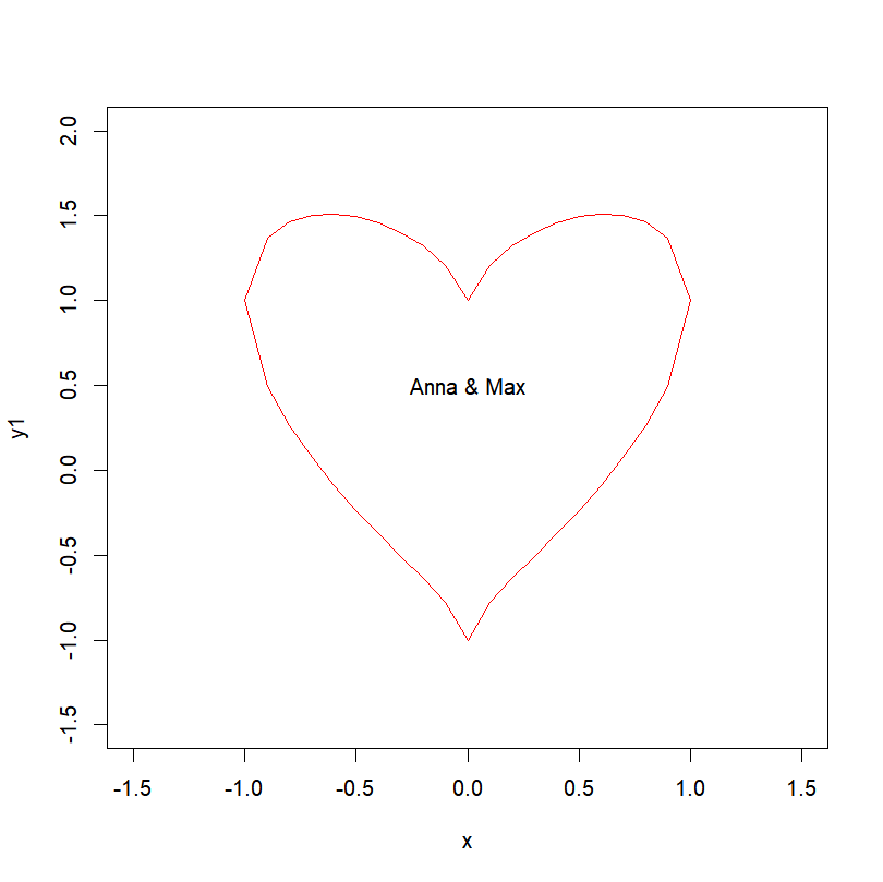
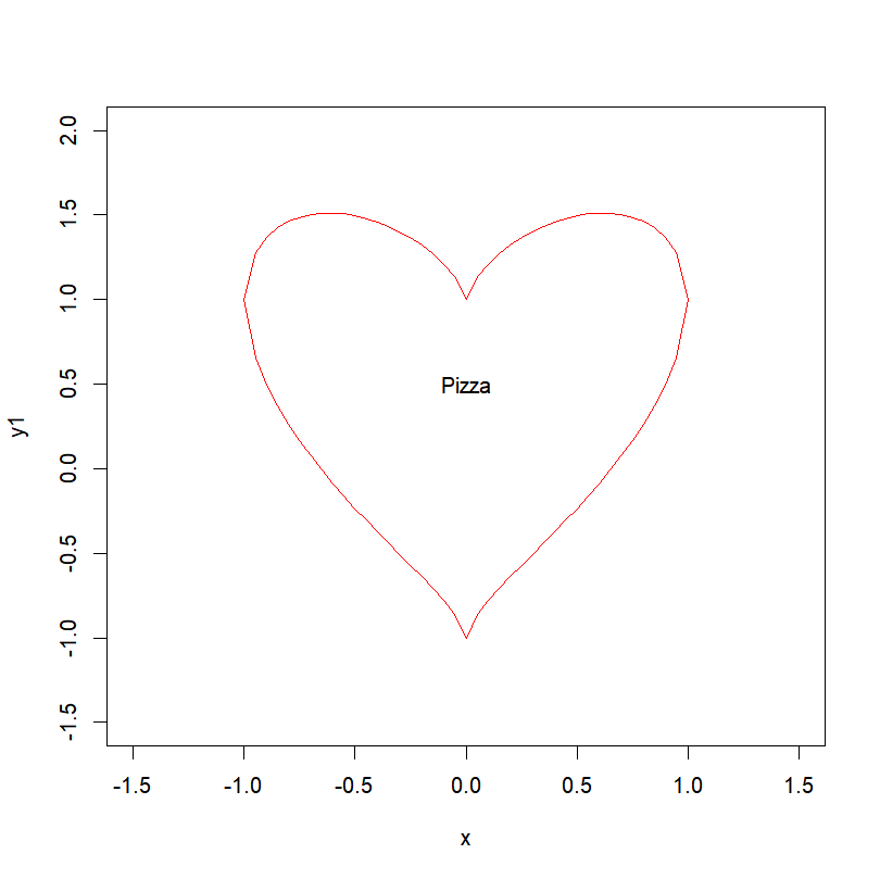
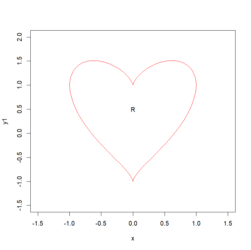
Exercise 5.4Create a function “jaimeR()” that: – takes as argument/input a vector ‘x’, and a character string “name” (with “name” set as ‘NULL’ by default) – creates 2 vectors ‘y1’ and ‘y2’ containing NA, and of the same length as ‘x’ – loops around all the values in x – tests if the value x[i] is between -1 and 1 – if x[i] is between -1 and 1, sets: y1[i] = sqrt(1-x[i]^2) + (x[i]^2)^(1/3) y2[i] = -sqrt(1-x[i]^2) + (x[i]^2)^(1/3) – else, sets: y1[i]=NA y2[i]=NA – plots ‘y1’ against x, with a red line, with the x-axis coordinates ranging from -1.5 to 1.5, and the y-axis coordinates ranging from -1.5 to 2 ( hint: set the arguments ‘xlim=c(-1.5,1.5)’ and ‘ylim=c(-1.5,2)’ ) – adds a red line to the existing graph plotting ‘y2’ against ‘x’ – adds the text specified in the argument “name” at the coordinates (0,0.5) With the function “seq()”, create a vector ranging from -5 to 5 (with an increment of 1), and feed it to your function “jaimeR()” with “name” set to your name. Try to run it with an input vector with smaller increments (0.1, 0.05 and 0.01 for example) Be in awe…
|