GLM

Generalized Linear Models

Concept

The linear models we used so far allowed us to try to find the relationship between a continuous response variable and explanatory variables. One way of understanding it is that the response variable is following a normal distribution which has a mean equal to a linear combination of the explanatory variables. Simply put, the response variable is equal to a linear combination of the covariates plus some random noise, and this random noise has normal distribution. This is one of the things we were checking with the Q-Q plot.

A generalization of this approach can be used when dealing with a response variable that is discrete and/or bounded. Three typical situations where this might occur:

1/ Binary: Trying to determine the probability of an event to happen. For example, one might want to model occupancy of a species of interest in a particular area (i.e. is it present or not). Our response variable would therefore be either a 0 or a 1. However, a linear regression could easily return values that are not contained in this set.

2/ Discrete and bounded: Trying to model the observation of a repeated binary event. For example, you might want to figure out what is the probability to detect an animal given that it is present in an area. To do so, you could conduct five 10-minute sessions where you will note during how many sessions the animal has been detected. Obviously, the amount of possible detection (binary event: detection or no detection) will be bounded between 0 and the total number of session (repeated measures). Or, you might be interested in the number of female nestlings in a nest in a study of sex ratio. The count can’t be more than the total clutch size in the nest. Moreover, there is no “half-detection”. I don’t care that you’re unsure if the howling you heard during session 3 was the wolf you are studying or a student caught in a bear trap, you can’t count it as a half-detection “just in case”. A regular linear model would not respect the bounding nor the fact that we have discrete values.

3/ Discrete: Trying to model a population’s abundance. We are counting individuals. Chances are that we are not going to find 0.24 or 17.2 or 82.7458 individuals. We are modeling a discrete number of individuals. The linear approach could not only give us half individuals in the regression, but could also lead us to predict negative numbers of individuals for certain values of the covariates.

We need a solution to accommodate those situations! Enter the GLMs! The Generalized Linear Models. (Normally, as you read that, The Ride of the Valkyries should be playing in your head.) GLMs are composed of three elements: a probability distribution, a link function and a linear predictor. The probability distribution illustrates the randomness in the response variable. The link function “links” the parameters controlling the probability distribution parameter(s) to the linear predictor. The linear predictor is a linear combination of covariates we hypothesize to be related to the response variable.

Distributions

As said above, the probability distribution is the part of the GLM that allows us to describe the randomness in the response. It will be different depending on the type of response we are observing.

The normal distribution – The linear models we have used so far aimed at estimating the mean of a normal distribution for the response variable by expressing it as a result of our covariates. The normal distribution has 2 parameters: the mean, and the standard deviation. We are simply expressing the mean of the normal distribution as a linear combination of our covariates to link our explanatory variables to our response variable!

The binomial distribution – The binomial distribution will be used when facing a) a binary variable (presence/absence, success/failure, yes/no) or b) the repetition of a binary variable (number of occupied sites in a given area for example). In situation a), only one parameter is necessary to model the response variable: the event probability. In case b), two parameters are necessary: the probability of a single event, and the number of repetition. As the number of repetition is simply equal to the total of “success” and “failure”, this information is contained in the data. This leaves us with one parameter to once again model our response variable, the probability. Cool, we now just need to find a way to express this probability as a linear combination of our covariates to link our explanatory variables to our response variable!

The Poisson distribution – The Poisson distribution will typically be used for population counts. It has only one parameter (‘lambda’), and makes the assumption that the mean and the variance are equal. Once again, cool, we now just need to find a way to express this mean as a linear combination of our covariates to link our explanatory variables to our response variable! The Poisson distribution is basically what would happen to a binomial distribution for a really low probability (rare events) but over a really large number of trials. As a matter of fact, if we take ‘n’ trials and a probability ‘p’ of the targeted event to happen, the Poisson distribution with a mean ‘np’ can be seen as a good approximation of the binomial distribution if ‘n’ is at least 20 and ‘p’ is smaller than or equal to 0.05, and as an excellent approximation if ‘n’ is greater than or equal to 100 and the product ‘n’ by ‘p’ is lower than or equal to 10. Need proof? Here:

  # Binomial distribution with 100 trials and a probability of success of 0.05
hist(rbinom(100000,100,0.05),col="yellow")
  # Poisson distribution with a mean of 100*0.05
hist(rpois(100000,lambda=100*0.05),add=T,col="#0000ff66")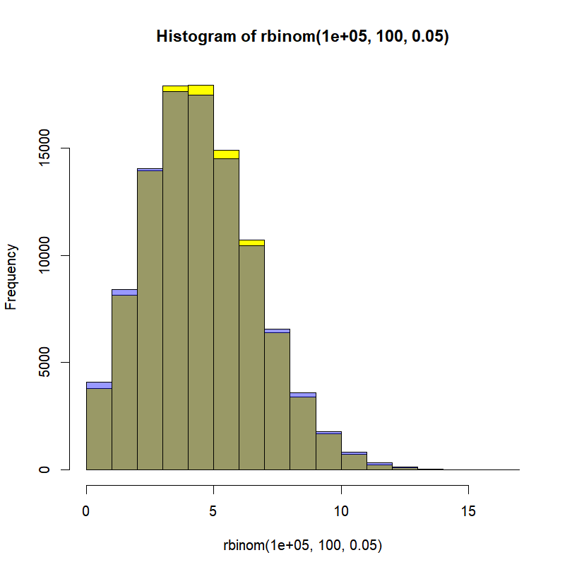

In yellow, the binomial distribution. In blue, the approximating Poisson distribution. In grey(ish) the overlap between the two. Not bad, right?

The link function

As you have hopefully understood, we now have different distributions available to provide a statistical framework for our response variable. We also have at least one parameter (e.g. mean, probability) for each distribution that controls it. We just need to find a function to link a linear combination of our explanatory variables to this parameter in order to model the relationship between the response variable and those covariates. This is what is called the link function.

The link function for the normal distribution is the identity function. Basically, it’s just the linear combination by itself, as we have always done so far.

The link function for the binomial distribution is the logit function. It allows to define a linear combination that varies between -Infinity and + Infinity and to transfer it on a 0 to 1 probability scale. For information, the logit of a probability ‘p’ is equal to the logarithm of the odds:

The link function for the Poisson distribution is the log function.

No need to worry too much about that right now, when we will specify the type of model we want to use to R, R will bundle the information about the probability distribution and the link function together. You just need to precise the family, and both the distribution and the corresponding link function will be selected.

The linear predictor

Now that we can link our response variable to the explanatory variables, we just need to define the linear predictor in the same way we have always done. And voila! We’ll be doing GLMs in no time. Let’s practice!

---

How to in practice

GLMs in R are performed with the function “glm()“. This function, as the linear regressions we have done so far, needs a model express through a formula and some data. One more argument needs to be specified: the family. The family is the description of the error distribution and link function to be used in the model. In practice, you will set this argument to “binomial” for a logistic regression, to “poisson” for a Poisson regression, and “gaussian” for a linear regression. More details and options about the families available are presented in the help of the “family()” function, but those should do the trick for the most common problems you will be facing. What about a couple of practical examples?

The linear regression

When the distribution probability used for the response variable is the normal distribution, a GLM is essentially a regular linear regression, such as the ones we have performed so far with the function “lm()”.

The logistic regression

The logistic regression is the GLM used when the response variable is the result of a binomial distribution and the link function is the logit function.

Let’s take for example the distribution of the spotted dahu (Dahutus maculosus dextrogyrus) in Northern Brittany, France. We studied the presence of the dahu on 10 hills. We went on each hill a different amount of times, and each time we recorded if we had been able to detect this elusive animal. We hypothesize that the presence of the dahu is related to the average slope of the hill. Here are the data:

data <-data.frame(
      # Site number
           sitenumber = 1:10,
      # Number of times detected on each site
           ndetect = c(1, 0, 3, 2, 3, 0, 6, 2, 3, 3),
      # Number of times not detected on each site
           nNOdetect = c(5, 6, 0, 2, 1, 4, 0, 2, 0, 1),
      # Standardized slope data for each site
           slope = c(-1.0365, -1.1277, 2.9394, 0.2728, 1.5166, -1.6598, 1.3249, 0.7227, 1.0143, 0.4275)
           )

First things first, let’s take a look at our data.

plot(ndetect~slope, data=data)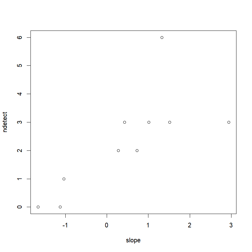

In order to conduct a logistic regression, we proceed as for the linear regression, but we also set the argument “family” to “binomial”:

dahu.res=glm(cbind(ndetect,nNOdetect)~slope,
             family=binomial,
             data=data)

We need to enter the response variable as a data frame with two columns, the first column corresponds to the detection, the second column to the non-detection. If I wanted to study a binary variable over several sites, I would simply have to enter a vector of 0 and 1 instead. If I have replicates, I have to enter a data frame with 2 columns.

A look at the results with the function “summary()“:

summary(dahu.res)
Call:
glm(formula = cbind(ndetect, nNOdetect) ~ slope, family = binomial,
    data = data)
Deviance Residuals:
     Min        1Q    Median        3Q       Max
-1.08294  -0.81103   0.02806   0.66110   1.14596
Coefficients:
            Estimate Std. Error z value Pr(>|z|)
(Intercept)  -0.4109     0.4906  -0.837  0.40238
slope         1.9383     0.5398   3.591  0.00033 ***
---
Signif. codes:  0 ‘***’ 0.001 ‘**’ 0.01 ‘*’ 0.05 ‘.’ 0.1 ‘ ’ 1
(Dispersion parameter for binomial family taken to be 1)
    Null deviance: 35.412  on 9  degrees of freedom
Residual deviance:  6.534  on 8  degrees of freedom
AIC: 19.733
Number of Fisher Scoring iterations: 5

As for the linear models we have used so far, R returns estimates of the model coefficients, and their statistical significance. Here, the intercept’s mean is -0.4109, but with an associated probability of 0.4028 is not statistically significant. The slope effect is 1.9383 and is highly significant. Estimates of the standard error around those means can be used to construct confidence intervals. We also get Akaike’s Information Criterion and model deviance, which are commonly used to choose between competing models.

We can also evaluate the overall performance of the model. The null deviance shows how well the response is predicted by a model with nothing but an intercept. This is essentially a chi square value on 9 degrees of freedom, and indicates very little fit (a highly significant difference between fitted values and observed values).

1-pchisq(35.412,9)
5.039208e-05

Adding in our predictor decreased the deviance by 28.878 (=35.412-6.534) points on 1 degree of freedom. The residual deviance is 6.534 on 8 degrees of freedom. We use this to test the overall fit of the model by once again treating this as a chi square value.

1-pchisq(6.534,8)
0.5876389

A chi square of 6.534 on 8 degrees of freedom yields a p-value of 0.5876389. The null hypothesis (i.e., the model) is not rejected. The fitted values are not significantly different from the observed values. The model including hills’ slope provides a good fit to our dahu observation data. 

As previously for the linear regression, if we want to plot the fitted line, we need to first get the results of the model (already done). Secondly, we need a data frame containing the values of the explanatory variables for which we are trying to predict the response variable.

slope.new <- seq(min(data$slope), max(data$slope), length.out = 100)
expl.pred=data.frame(slope=slope.new)

And finally, we use the “predict()” function with the model results and predictive variables. In the case of GLMs, the predicted response values are returned on the scale of the linear predictors (i.e. here the probabilities on logit scale, the log-odds). If we want to plot them, we will need to indicate the function that we want to have our predictions on the same scale as the response variable (i.e. the ratio of “success” over the total number of trials). This is achieved by setting the argument “type” to the value “response”. The predict function now returns the success response probability in function of the explanatory variable.

resp.pred <- predict(dahu.res, newdata=expl.pred, type="response")

Now, we just have to plot all of that. Remember that the predict function return fitted results on the probability scale, and therefore we need to plot the ratio of detection over the total number of sampling occasion (instead of simply the number of detections) in function of the covariate. The function “title()” is used to add a title and possibly other elements to a graph (more details on that in the next section).

plot(ndetect/(ndetect+nNOdetect) ~ slope, data=data)
lines(resp.pred ~ expl.pred$slope,col="red")      # Fitted values
title(main="Dahu detection rate with Fitted Logistic Regression Line")

We can easily compute and add the prediction’s 95% confidence interval. To do so, first we compute the predicted values on the linear scale, and ask for the corresponding standard errors.

pred.linkscale <- predict(dahu.res, newdata=expl.pred, se=T)

From there, we can approximate the 95% confidence interval on the linear scale, following the formula “95CI= mean +/- 1.96*SE” (formula based on the normal distribution, assuming that the residuals are normally distributed on the linear scale).

# Lower CI 95%
pred.linkscale.CI2.5=pred.linkscale$fit-1.96*pred.linkscale$se.fit
# Upper CI 95%
pred.linkscale.CI97.5=pred.linkscale$fit+1.96*pred.linkscale$se.fit 

Let’s back-transform from the linear scale to the response scale. To do that, we can feed the predicted values on the linear scale to the inverse link function. It’s possible to access the family used in the analysis with the function “family()”. This function takes as argument the object containing the GLM results, and returns (among other things) the inverse link function in the element “linkinv”.

pred.respScale.CI=data.frame(
                    CI2.5=family(dahu.res)$linkinv(pred.linkscale.CI2.5),
                    CI97.5=family(dahu.res)$linkinv(pred.linkscale.CI97.5)
                             )

What’s left to do? Simply plot the corresponding lines!

# Lower CI 95%
lines(pred.respScale.CI$CI2.5~expl.pred$slope,lty="dashed")
# Upper CI 95%
lines(pred.respScale.CI$CI97.5~expl.pred$slope,lty="dashed")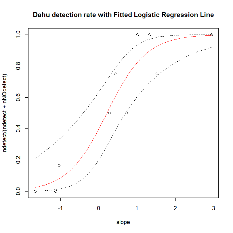 

Not too shabby, is it?

The Poisson regression

The Poisson regression is the GLM used when the response variable is the result of a -guess what- Poisson distribution and the link function is the log function. As previously stated, this is typically what you will use for population counts.

Let’s take for example the fish abundance off the coast of Cabot Cove. We have sample the fish population in 100 different sites and for each site we recorded the total abundance and the amount of food available. We hypothesize that fish abundance is related to the food availability. Here are the data:

fish.data=data.frame(sitenumber=1:100,
                 fish.population=c(7, 3, 7, 1, 9, 1, 0, 0, 33, 15, 0, 8, 10, 6,
                     6, 0, 5, 4, 0, 0, 18, 1, 0, 4, 9, 35, 7, 6, 52,
                     18, 2, 6, 0, 1, 1, 1, 17, 0, 1, 0, 1, 2, 3, 2,
                     1, 5, 21, 5, 3, 2, 0, 2, 12, 4, 0, 0, 3, 0, 0,
                     2, 4, 10, 13, 10, 2, 4, 15, 3, 4, 20, 2, 1, 33,
                     0, 3, 0, 6, 32, 15, 0, 18, 5, 1, 1, 1, 0, 0, 52,
                     2, 23, 0, 4, 8, 4, 6, 13, 4, 0, 0, 3),
            # Standardized food availability
                 food=c(0.7726, 0.3052, 0.4091, -0.7749, 0.9618, -0.2377, -1.2015,
                       -0.8639, 1.6418, 1.1006, -1.2936, 0.3786, 0.5588, 0.3441, 0.4137,
                       -0.625, 0.5609, -0.2873, -0.7354, -2.353, 1.3576, 0.0096, -1.6573,
                        0.5267, 0.9805, 1.5259, 0.4241, 0.5559, 1.9227, 1.1616, -0.4877,
                        0.434, -1.3075, -1.2571, -0.4045, 0.3146, 1.0496, -1.1584, -0.9643,
                       -0.7425, -0.6268, -0.2768, -0.0564, 0.0732, -0.4332, 0.7553,
                        1.2763, 0.5868, 0.0771, -0.2776, -0.1421, -0.5285, 0.8199, 0.11,
                       -0.4764, -1.189, 0.3835, 0.1221, -0.327, -0.4722, 0.4809, 0.9963,
                        0.8434, 0.9199, -0.2348, 0.308, 1.0344, 0.0919, -0.0676, 1.317,
                       -0.2041, -0.4657, 1.565, -0.8463, 0.457, -1.1507, 1.0512, 1.7268,
                        1.0127, -0.4697, 1.4311, 0.1237, -0.8073, -0.6794, -0.8374, -0.053,
                       -1.2292, 1.8966, -0.3192, 1.4033, -0.6946, 0.1261, 1.1178, -0.0309,
                        0.9486, 0.9798, -0.4686, -1.9257, -1.4116, -0.1264)
                        )

Quick look:

plot(fish.population~food,fish.data)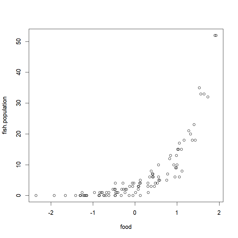

Want to do a Poisson regression? No worries mate, you just use the “glm()” function and set the argument “family” to “Poisson” (go figure…):

fish.res=glm(fish.population~food,
             family=poisson,
             data=fish.data)

As usual, to get a summary of our model’s results, we use the well-named function “summary()”.

summary(fish.res)
Call:
glm(formula = fish.population ~ food, family = poisson, data = fish.data)
Deviance Residuals:
     Min        1Q    Median        3Q       Max
-2.41700  -0.82552  -0.00656   0.59693   2.08337
Coefficients:
            Estimate Std. Error z value Pr(>|z|)
(Intercept)  0.87677    0.07580   11.57   <2e-16 ***
food         1.59823    0.05891   27.13   <2e-16 ***
---
Signif. codes:  0 ‘***’ 0.001 ‘**’ 0.01 ‘*’ 0.05 ‘.’ 0.1 ‘ ’ 1
(Dispersion parameter for poisson family taken to be 1)
    Null deviance: 1090.685  on 99  degrees of freedom
Residual deviance:   92.837  on 98  degrees of freedom
AIC: 365.86
Number of Fisher Scoring iterations: 5

First things first, how is the model fitting? The Null deviance and the corresponding degrees of freedom indicate a highly significant difference between fitted values and observed values:

1-pchisq(fish.res$null.deviance,fish.res$df.null)
0

Noticed how I directly extracted the “null.deviance” and the number of degrees of freedom “df.null” from the GLM output?

Once the predictor is added, it’s a different story!

1-pchisq(fish.res$deviance,fish.res$df.residual)
0.6283983

Now, the fitted values are not significantly different from the observed values. We therefore cannot reject the null hypothesis, i.e. the model.

We also see here that we have statistically significant intercept and food effect. We can also directly extract the corresponding coefficient values from the GLM output:

fish.res$coefficients
(Intercept)        food
  0.8767657        1.5982324

This is a list from which we can extract the coefficient on the log-scale for our food effect.

fish.res$coefficients[["food"]]
1.598232

Which in turn can be used to express our population growth rate depending on the food availability. Since this coefficient is on the log scale, we need to use the inverse function of the log, i.e. the exponential, in order to get this information.

exp(fish.res$coefficients[["food"]])
4.944285

Every time we add one food unit on the standardized scale, the fish population will be 4.9 times larger. In a real life situation, we would also back transform the standardized covariate “food” to give a clearer ecological description of our dynamic.

And, as for the previous fitted models, we can plot the fitted line in the following way:

food.new <- seq(min(fish.data$food), max(fish.data$food), length.out = 100)     # Creating new values of the covariates for which we want to predict the response variable
expl.pred=data.frame(food=food.new)
resp.pred <- predict(fish.res, newdata=expl.pred, type="response")          # Predictions
plot(fish.population~ food, data=fish.data)
lines(resp.pred ~ expl.pred$food,col="red")      # Fitted values
title(main="Fish abundance depending on food resources \n with Fitted Poisson Regression Line")

And compute and plot the prediction’s 95% confidence interval:

pred.linkscale <- predict(fish.res, newdata=expl.pred, se=T)
pred.linkscale.CI2.5 = pred.linkscale$fit-1.96*pred.linkscale$se.fit
pred.linkscale.CI97.5 = pred.linkscale$fit+1.96*pred.linkscale$se.fit
pred.respScale.CI=data.frame(
                   CI2.5=family(fish.res)$linkinv(pred.linkscale.CI2.5),
                   CI97.5=family(fish.res)$linkinv(pred.linkscale.CI97.5))
lines(pred.respScale.CI$CI2.5 ~ expl.pred$food,lty="dashed")
lines(pred.respScale.CI$CI97.5 ~ expl.pred$food,lty="dashed")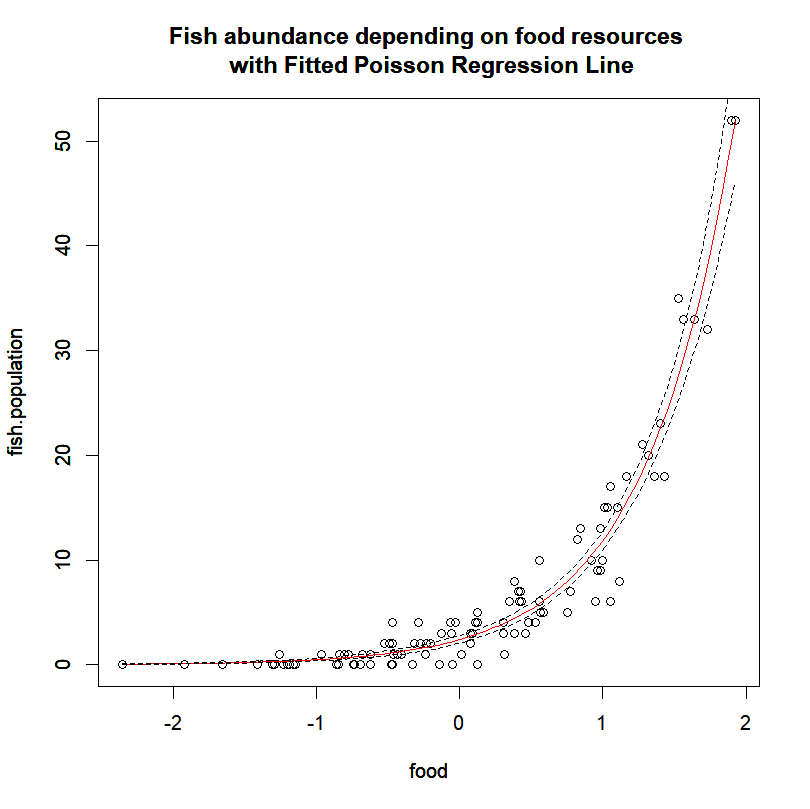

I know… Beautiful, right?

Finally, no matter what type of GLM is used, different combination of explanatory variables will provide different fit for the data. Models will need to be selected in order to find a good trade-off between the number of parameters used and the fit. Model selection is beyond the scope of this introduction to R, but know that it can be done really easily in R, for example through the use of the function “step()“. For more information on how to proceed, you can simply check its help file.